Download
1 / 34
340 likes | 364 Vues
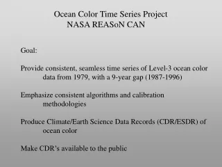
The goal of the Ocean Color Time Series Project is to provide consistent and seamless time series of Level-3 ocean color data from 1979, with a 9-year gap (1987-1996). The project emphasizes consistent algorithms and calibration methodologies to produce Climate/Earth Science Data Records (CDR/ESDR) of ocean color and make them available to the public.

E N D
Ocean Color Time Series Project NASA REASoN CAN Goal: Provide consistent, seamless time series of Level-3 ocean color data from 1979, with a 9-year gap (1987-1996) Emphasize consistent algorithms and calibration methodologies Produce Climate/Earth Science Data Records (CDR/ESDR) of ocean color Make CDR’s available to the public
CDR: A time series of sufficient length, consistency, and continuity to determine climate variability and change National Research Council, 2004 Technical Definition of Consistent/Seamless: all temporal sensor artifacts removed no obvious interannual discontinuities unattributable to natural variability all known mission-dependent biases removed or quantified similar data quality and structure
VIIRS-2 Ocean Color Satellite Missions: 1978-2010 and Beyond VIIRS-NPP MODIS-Aqua MODIS-Terra CZCS SeaWiFS OCTS/ POLDER “Missions to Measurements” 1980 1990 2000 2010
Ocean Color Time Series REASoN CAN Team: Watson Gregg, NASA/Global Modeling and Assimilation: Oversight, Data Analysis DAAC: Data Access and Visualization, Archival, Distribution Jim Acker, NASA/GES-DAAC Steve Kempler, NASA/GES-DAAC Greg Leptoukh, NASA/GES-DAAC OBPG: Data Processing, In Situ Data Collection, Coincident Data Merging Gene Feldman, NASA/Ocean Color Processing Chuck McClain, NASA/Ocean Color Processing UCSB: Coincident Data Merging/ Data Technology Jim Frew, Stephane Maritorena, David Siegel
Consistent Ocean Color Time Series Requires Similar • 1) Calibration • 2) Algorithms • Spatial and Temporal Resolution (Level-3) • 4) Data Format • 5) Access • Analysis Tools • 7) Bias characterization
SST: increased 0.2oC in 20 years = 1% change, or 0.05%/year Estimated from Reynolds using AVHRR SeaWiFS: Maximum difference over lifetime (highest annual mean – lowest annual mean) = 5% Surface Air Temperature: increased 1oC in 100 years = 5% change, or 0.05%/year Estimated from thermometers, tree rings, ice boreholes
The REASoN Project has now completed data records for OCTS (RV1) SeaWiFS (V5.1) MODIS-Aqua (V1.1) using consistent processing methodologies as defined
Regional Annual Trends SeaWiFS SeaWiFS/Aqua Linear trends using 7-year average/composite images were calculated, and when significant (P < 0.05), shown here.
OCTS Nearly constant offset: about 15% + 1.5%
NASA Ocean Biogeochemical Model (NOBM) Chlorophyll,Phytoplankton Groups Primary Production Nutrients DOC, DIC, pCO2 Spectral Irradiance/Radiance Outputs: Winds, ozone, relative humidity, pressure, precip. water, clouds (cover, τc), aerosols (τa, ωa, asym) Dust (Fe) Sea Ice Winds SST Radiative Model (OASIM) Ed(λ) Es(λ) Ed(λ) Es(λ) IOP Layer Depths Biogeochemical Processes Model Circulation Model (Poseidon) Temperature, Layer Depths Advection-diffusion Global model grid: domain: 84S to 72N1.25 lon., 2/3 lat.14 layers
Trends 1998-2004 Data/Model Linear Annual Trend SeaWiFS -0.71% ns NOBM Free Run 0.18% ns NOBM assimilation SeaWiFS -0.98% ns
Compared to In situ Data Bias Uncertainty N SeaWiFS -1.3% 32.7% 2086 Free-run Model -1.4% 61.8% 4465 Assimilation Model 0.1% 33.4% 4465
Advantages of Data Assimilation Achieves desired consistency, with low bias Responds properly to climatic influences Full daily coverage – no sampling error Effective use of data to keep model on track Only spatial variability required from sensors Disadvantages of Data Assimilation Low resolution (for now) No coasts (for now) Excessive reliance on model biases Cannot validate model trends with sensor data
Can the CZCS provide a Climate Data Record? CDR: A time series of sufficient length, consistency, and continuity to determine climate variability and change National Research Council, 2004
CZCS The most ground breaking biological satellite in history More than 1000 peer-reviewed publications Major scientific advances Unprecedented view of spatial variability (gyres, coasts) Immenseness of the North Atlantic spring bloom Iron hypothesis Validation of first ocean biology models Importance of CDOM, aerosols, Case 1 and Case 2 waters Warm core rings, cold core rings Associations between tuna populations and fronts First data-driven estimates of global primary production First attempts at biological satellite data assimilation Established chlorophyll as a climate variable
CZCS Deficiencies 1) Low SNR 2) 5 bands, only 4 of which quantitatively useful -- limits aerosol detection capability 3) Navigation 4) Polarization 5) El Chichon 6) Anomalous behavior post-1981 7) Sampling
410 412 411 411 412 443 443 443 442 442 445 490 488 488 488 490 520 520 510 531 531 550 565 555 551 551 555 670 670 670 667 667 672 765 765 746 746 746 865 865 846 846 865 Ocean Color Missions: Bands CZCS OCTS SeaWiFS Terra Aqua VIIRS 410 nm 443 nm 490 nm 510 nm 555 nm 670 nm 765 nm 865 nm
CZCS Aerosol Workarounds Evans and Gordon, 1994, JGR Fixed aerosol type (epsilon) Advantages: simple to implement led to data access, major advances in knowledge Disadvantages: all variability assumed to be oceanic in origin single scattering aerosols underestimates of chlorophyll Gregg et al., 2002 Applied Optics Characterize aerosols in clear water, extrapolate using statistical 2-D methods (objective analysis), access SeaWiFS multiple scattering tables Advantages: coincident variability partitioned among aerosols and ocean preserves knowledge derived from actual data 2-D objective extrapolation multiple scattering aerosols clear water represents approx. 90% of oceans Disadvantages: extrapolation is statistical requires aerosol fronts and chlorophyll fronts are uncorrelated
Antoine et al., 2005, JGR Iterate between pre-defined optical representation in the ocean (Morel ocean) and atmosphere (Angstrom atmosphere) to obtain numerical convergence Advantages: coincident preserves knowledge derived from actual data variability partitioned among aerosols and ocean Disadvantages: single scattering aerosols only works in optically well-behaved areas REASoN V2, Sep. 2006 Fixed aerosol model (maritime 99% humidity), CZCS-derived multiple scattering tables Advantages: simple to implement multiple scattering aerosols Disadvantages: all variability assumed to be oceanic in origin
1989 data set CZCS Navigation Gregg et al., 2002
CZCS Polarization Exists, and is tilt-dependent Gordon: band-to-band polarization is removed through in situ calibration residual tilt-dependent polarization is maximum <1 digital count
El Chichon Massive volcanic eruptions, late March 1982, early April 1982 (2)
Gordon and Castano 1988: up to tau = 0.4, effect = 1-2 digital counts at La(443) Comparisons with In situ Data in Spring RMS Bias
All missions have “events” SeaWiFS: 3 El Ninos (1997-1998; 2002-2003; now) 1 major 2.5-year La Nina (1998-2000) 26 named tropical storms/hurricanes 2005 (overall increased frequency and intensity of hurricanes) Canadian wildfires 2002 Indonesian wildfire 1997 Largest fires in history in Alaska 2004 Biomass burning in Africa and South America Asian Brown Cloud Great Saharan Dust Storm 2004, 2006
Time Series Issues • How calibrate historical and future sensors, maintaining consistency? • 2) Is BRDF a good idea? • 3) Can we define more rigorous metrics than in situ comparisons, that • constrain global mean estimates? • 4) Is it acceptable to have two data streams: • operational (best available methods; mission-dependent) • climate (maximum commonality/consistency of methods)? • 5) How much consistency can we achieve without resorting to post- • processing methods (blending of in situ data, assimilation)? • Is this necessary?