Chi-squared Tests
Chi-squared Tests. We want to test the “goodness of fit” of a particular theoretical distribution to an observed distribution. The procedure is:. 1. Set up the null and alternative hypotheses and select the significance level.

Chi-squared Tests
E N D
Presentation Transcript
We want to test the “goodness of fit” of a particular theoretical distribution to an observed distribution. The procedure is: • 1. Set up the null and alternative hypotheses and select the significance level. • 2. Draw a random sample of observations from a population or process. • 3. Derive expected frequencies under the assumption that the null hypothesis is true. • 4. Compare the observed frequencies and the expected frequencies. • 5. If the discrepancy between the observed and expected frequencies is too great to attribute to chance fluctuations at the selected significance level, reject the null hypothesis.
Example 1: Five brands of coffee are taste-tested by 1000 people with the results below. Test at the 5% level the hypothesis that, in the general population, there is no difference in the proportions preferring each brand (i.e.: H0: pA= pB= pC= pD= pE versus H1: not all the proportions are the same).
If all the proportions were the same, we’d expect about 200 people in each group, if we have a total of 1000 people.
We next compute the differences in the observed and theoretical frequencies.
Then we divide each of the squares by the expected frequency and add the quotients. The resulting statistic has a chi-squared (2) distribution.
f(2) 2 The chi-squared (2) distribution The chi-squared distribution is skewed to the right. (i.e.: It has the bump on the left and the tail on the right.)
In these goodness of fit problems, the number of degrees of freedom is: In the current problem, we have 5 categories (the 5 brands). We have 1 restriction. When we determined our expected frequencies, we restricted our numbers so that the total would be the same total as for the observed frequencies (1000). We didn’t estimate any parameters in this particular problem. So dof = 5 – 1 – 0 = 4 .
f(2) 2 Large values of the 2 statistic indicate big discrepancies between the observed and theoretical frequencies. So when the 2 statistic is large, we reject the hypothesis that the theoretical distribution is a good fit. That means the critical region consists of the large values, the right tail. acceptance region crit. reg.
From the 2table, we see that for a 5% test with 4 degrees of freedom, the cut-off point is 9.488. In the current problem, our 2 statistic had a value of 136.49. So we reject the null hypothesis and conclude that the proportions preferring each brand were not the same. f(2) acceptance region 0.05 crit. reg. 9.488 136.49
Example 2: A diagnostic test of mathematics is given to a group of 1000 students. The administrator analyzing the results wants to know if the scores of this group differ significantly from those of the past. Test at the 10% level.
Based on the historical relative frequency, we determine the expected absolute frequency, restricting the total to the total for the current observed frequency.
We subtract the theoretical frequency from the observed frequency.
We divide the square by the theoretical frequency and sum up.
We have 5 categories (the 5 grade groups). We have 1 restriction. We restricted our expected frequencies so that the total would be the same total as for the observed frequencies (1000). We didn’t estimate any parameters in this particular problem. So dof = 5 – 1 – 0 = 4 .
From the 2table, we see that for a 10% test with 4 degrees of freedom, the cut-off point is 7.779. In the current problem, our 2 statistic had a value of 125. So we reject the null hypothesis and conclude that the grade distribution is NOT the same as it was historically. f(2) acceptance region 0.10 crit. reg. 7.779 125
Example 3: Test at the 5% level whether the demand for a particular product as listed below has a Poisson distribution.
Multiplying the number of days on which each amount was sold by the amount sold on that day, and then adding those products, we find that the total number of units sold on the 200 days is 600. So the mean number of units sold per day is 3.
We use the 3 as the estimated mean for the Poisson distribution. Then using the Poisson table, we determine the probabilities for each x value.
Then we multiply the probabilities by 200 to compute ft, the expected number of days on which each number of units would be sold. By multiplying by 200, we restrict the ft total to be the same as the fo total.
When the ft’s are small (less than 5), the test is not reliable. So we group small ft values. In this example, we group the last 4 categories.
Next we subtract the theoretical frequencies ft from the observed frequencies fo.
We have 8 categories (after grouping the small ones). We have 1 restriction. We restricted our expected frequencies so that the total would be the same total as for the observed frequencies (200). We estimated 1 parameter, the mean for the Poisson distribution. So dof = 8 – 1 – 1 = 6 .
From the 2table, we see that for a 5% test with 6 degrees of freedom, the cut-off point is 12.592. In the current problem, our 2 statistic had a value of 5.53. So we accept the null hypothesis that the Poisson distribution is a reasonable fit for the product demand. f(2) acceptance region 0.05 crit. reg. 5.53 12.592
Example 4: Test at the 10% level whether the following exam grades are from a normal distribution. Note: This is a very long problem.
If the distribution is normal, we need to estimate its mean and standard deviation.
To estimate the mean, we first determine the midpoints of the grade intervals.
We then multiple these midpoints by the observed frequencies of the intervals, add the products, and divide the sum by the number of observations. The resulting mean is 7500/100 = 75.
Next we need to calculate the standard deviation We begin by subtracting the mean of 75 from each midpoint, and squaring the differences.
We multiply by the observed frequencies and sum up. Dividing by n –1 or 99, the sample variance s2 = 149.49495. The square root is the sample standard deviation s = 12.2268.
We will use the 75 and 12.2268 as the mean and the standard deviation of our proposed normal distribution. We now need to determine what the expected frequencies would be if the grades were from that normal distribution.
.3907 .1093 0 -1.23 Z Start with our lowest grade category, under 60. We then expect that 10.93% of our 100 observations, or about 11 grades, would be in the lowest grade category. So 11 will be one of our ft values. We need to do similar calculations for our other grade categories.
.1591 .3907 0 -1.23 -0.41 Z The next grade category is [60,70). So 23.16% of our 100 observations, or about 23 grades, are expected to be in that grade category.
.1591 .1591 0 -0.41 0.41 Z The next grade category is [70,80). So 31.82% of our 100 observations, or about 32 grades, are expected to be in that grade category.
.1591 .3907 0 Z 0.41 1.23 The next grade category is [80,90). So 23.16% of our 100 observations, or about 23 grades, are expected to be in that grade category.
.3907 .1093 0 1.23 Z The highest grade category is 90 and over. So 10.93% of our 100 observations, or about 11 grades, are expected to be in that grade category.
Now we can finally compute our 2 statistic. We put in the observed frequencies that we were given and the theoretical frequencies that we just calculated.
We subtract the theoretical frequencies from the observed frequencies, square the differences, divide by the theoretical frequencies, and sum up. The resulting 2 statistic is 4.3104.
We have 5 categories (the 5 grade groups). We have 1 restrictions. We restricted our expected frequencies so that the total would be the same total as for the observed frequencies (100). We estimated two parameters, the mean and the standard deviation. So dof = 5 – 1 – 2 = 2 .
From the 2table, we see that for a 10% test with 2 degrees of freedom, the cut-off point is 4.605. In the current problem, our 2 statistic had a value of 4.31. So we accept the null hypothesis that the normal distribution is a reasonable fit for the grades. f(2) acceptance region 0.10 crit. reg. 4.31 4.605
We can also use the 2 statistic to test whether two variables are independent of each other.
Example 5: Given the following frequencies for a sample of 10,000 households, test at the 1% level whether the number of phones and the number of cars for a household are independent of each other.
and the row and column percentages (marginal probabilities).
Recall that if 2 variables X and Y are independent of each other, then Pr(X=x and Y=y) = Pr(X=x) Pr(Y=y)


