Download
1 / 40
410 likes | 620 Vues
Marine Geospatial Ecology Tools Open Source Geoprocessing for Marine Ecology. Jason Roberts, Ben Best, Dan Dunn, Eric Treml, Pat Halpin Duke University Marine Geospatial Ecology Lab 4-Mar-2009. Talk outline. Overview of MGET Quick tour of the MGET tool collection

E N D
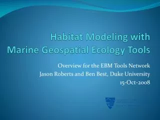
Marine Geospatial Ecology ToolsOpen Source Geoprocessing for Marine Ecology Jason Roberts, Ben Best, Dan Dunn, Eric Treml, Pat Halpin Duke University Marine Geospatial Ecology Lab 4-Mar-2009
Talk outline • Overview of MGET • Quick tour of the MGET tool collection • Example application: habitat modeling
Also useful for terrestrial problems! What is MGET? • A collection of geoprocessing tools for marine ecology • Oceanographic data management and analysis • Habitat modeling, connectivity modeling, statistics • Highly modular; designed to be used in many scenarios • Emphasis on batch processing and interoperability • Free, open source software • Written in Python, R, MATLAB, C#, and C++ • Minimum requirements: Win XP, Python 2.4 • ArcGIS 9.1 or later currently needed for many tools • ArcGIS and Windows are only non-free requirements
Visualize scenarios Develop conceptual models Collect physical, biological, and socioeconomic data Set goals & priorities Analyze data & develop models and scenarios Make & implement EBM decisions Monitor & assess
Visualize scenarios Develop conceptual models Conceptual modeling tools Collect physical, biological, and socioeconomic data Data collection and management tools Data processing tools Stakeholder communication & engagement tools Set goals & priorities • Modeling tools • Model development tools • Watershed models • Dispersal and habitat models • Marine ecosystem models • Social science models Scenario visualization tools Analyze data & develop models and scenarios • Sector-specific decision support tools • Conservation and restoration site selection • Coastal zone management tools • Fisheries management tools • Hazard assessment and resiliency planning tools • Land use planning tools Make & implement EBM decisions Monitor & assess Monitoring & assessment tools Project management tools
Visualize scenarios Develop conceptual models Conceptual modeling tools Collect physical, biological, and socioeconomic data Data collection and management tools Data collection and management tools Data processing tools Data processing tools Stakeholder communication & engagement tools MGET Set goals & priorities • Modeling tools • Model development tools • Watershed models • Dispersal and habitat models • Marine ecosystem models • Social science models • Modeling tools • Model development tools • Watershed models • Dispersal and habitat models • Marine ecosystem models • Social science models Scenario visualization tools Analyze data & develop models and scenarios • Sector-specific decision support tools • Conservation and restoration site selection • Coastal zone management tools • Fisheries management tools • Hazard assessment and resiliency planning tools • Land use planning tools Make & implement EBM decisions Monitoring & assessment tools Monitor & assess Project management tools
MGET’s software architecture MGET “tools” are really just Python functions, e.g.: defMyTool(input1, input2, input3, output1) MGET exposes them to several types of external callers:
MGET interface in ArcGIS The MGET toolbox appears in the ArcToolbox window
MGET interface in ArcGIS • Drill into the toolbox to find the tools • Double-click tools to execute directly, or drag to geoprocessing models to create a workflow
Integration The Python functions can invoke C++, MATLAB, R, ArcGIS, and COM classes.
MGET utilizes a lot of other software Interpreters / Runtimes Python MATLAB Component Runtime R Python Packages docutils httplib2 lxml netcdf4 numpy osgeo pydap pyparsing pyproj pywin32 rpy setuptools C Libraries GDAL/OGR gzip hdf libxml libxslt netcdf proj4 zlib Applications ArcGIS NOAA CoastWatch Utilities R Packages gam MASS mgcv rgdal ROCR All but one of these (pywin32) are installed automatically
Analyzing larval connectivity Ocean currents data Larval density time series rasters Coral reef ID and % cover maps Tool downloads data for the region and dates you specify Edge list feature class representing dispersal network Original research by Eric A. Treml
Batch processing Copy one raster at a time
Batch processing Copy rasters that you list in a table
Batch processing Copy rasters from a directory tree
Tools for specific products Downloads sea surface height data from http://opendap.aviso.oceanobs.com/thredds
AVHRR Daytime SST 03-Jan-2005 Identifying SST fronts Mexico Cayula and Cornillion (1992) edge detection algorithm Step 1: Histogram analysis ArcGIS model Bimodal Optimal break 27.0 °C Frequency Temperature Example output 28.0 °C Step 2: Spatial cohesion test Front Mexico 25.8 °C Strong cohesion front present Weak cohesion no front ~120 km
Identifying geostrophic eddies Available in MGET 0.8 SSH anomaly Example output Aviso DT-MSLA 27-Jan-1993 Red: Anticyclonic Blue: Cyclonic Negative W at eddy core
Example application: habitat modeling Probability of occurrence predicted from environmental covariates Presence/absence observations Multivariate statistical model Sampled environmental data Binary classification Bathymetry SST Warning: Habitat modeling is complicated! This simplified example is meant to briefly illustrate tools. Consult the literature for best practices! Chlorophyll
Focal species: Stenella frontalis Common name: Atlantic Spotted Dolphin Photo: Garth Mix Distribution: Tropical and warm temperate Atlantic Study area: Eastern U.S. Map: OBIS-SEAMAP
Species observation data The Ocean Biogeographic Information System (OBIS) is a global database of marine species observations. The OBIS-SEAMAP system at Duke University holds the records for seabirds, marine mammals, and sea turtles, including records gathered during NOAA cruises.
Environmental predictor variables Bathymetry: ETOPO2V2 from NOAA NGDC SST: Monthly climatological 4km AVHRR Pathfinder from NOAA NODC Chlorophyll: Monthly climatologicalSeaWiFS chlorophyll-a from NASA GSFC Images shown above are for month of March
Step 1: Download species points Download points using MGET tool: • Presence: Records of Stenella frontalis • Absence: Records of other cetaceans The tool uses the DiGIR protocol to retrieve data from OBIS servers
Red: Presence Green: Absence
Step 2: Convert oceanography to Arc rasters • Download with FTP from NOAA and NASA: • ETOPO2 bathymetry – 1 binary file • AVHRR Pathfinder monthly climatological SST – 12 HDF files • SeaWiFSmonthly climatological chlorophyll – 12 HDF files • Convert to ArcGIS rasters using MGET tools:
Step 3: Sample oceanography at points • Need to sample rasters and populate fields • Must sample SST and chlorophyll by date
Step 3: Sample oceanography at points Sampling bathymetry is easy because it is static To sample dynamic data such as SST and chlorophyll, you must first calculate the paths to rasters to sample from the points’ dates Then use an MGET batch sampling tool
Step 4: Create exploratory plots Best predictors: SST and Chl
Step 5: Fit, evaluate, and predict model Presence ~ s(SST) + s(log10(Chlorophyll))
Partial plots produced by the Fit GAM tool s(SST,8.97) s(log10(Chlorophyll),5.6) SST log10(Chlorophyll) SST Presence more likely at higher SST Presence more likely at lower Chl
The ROC plot ROC summary stats for cutoff: Model summary statistics: Area under the ROC curve (auc) = 0.960779 Mean cross-entropy (mxe) = 0.030566 Precision-recall break-even point (prbe) = 0.001866 Root-mean square error (rmse) = 0.087781 Contingency table for cutoff = 0.019638: Actual P Actual N Total Predicted P 287 3541 3828 Predicted N 26 32408 32434 Total 313 35949 36262 Accuracy (acc) = 0.901633 Error rate (err) = 0.098367 Rate of positive predictions (rpp) = 0.105565 Rate of negative predictions (rnp) = 0.894435 True positive rate (tpr, or sensitivity) = 0.916933 False positive rate (fpr, or fallout) = 0.098501 True negative rate (tnr, or specificity) = 0.901499 False negative rate (fnr, or miss) = 0.083067 Positive prediction value (ppv, or precision) = 0.074974 Negative prediction value (npv) = 0.999198 Prediction-conditioned fallout (pcfall) = 0.925026 Prediction-conditioned miss (pcmiss) = 0.000802 Matthews correlation coefficient (mcc) = 0.246384 Odds ratio (odds) = 101.026394 SAR = 0.650065 Cutoff = 0.020 True positive rate False positive rate By default, tool selects the cutoff closest to the point of perfect classification (0, 1)
Rasters output by the Predict GAM tool Predicted presence: Range: 0 - 0.25 Standard errors: Range: 0 - 0.11 Binary classification: Species range map produced by classifying presence into 0 or 1 according to ROC cutoff Similar to OBIS-SEAMAP range map? Predictions for October
Acknowledgements A special thanks to the many developers of the open source software that MGET is built upon, including: Guido van Rossum and his many collaborators; Mark Hammond; Travis Oliphant and his collaborators; Walter Moreira and Gregory Warnes; Peter Hollemans; David Ullman, Jean-Francois Cayula, and Peter Cornillon; Stephanie Henson; Tobias Sing, Oliver Sander, NikoBeerenwinkel, and Thomas Lengauer; Frank Warmerdam and his collaborators, Howard Butler; Timothy H. Keitt, Roger Bivand, EdzerPebesma, and Barry Rowlingson; Gerald Evenden; Jeff Whitaker; Roberto De Almeida and his collaborators; Joe Gregorio; David Goodger and his collaborators; Daniel Veillard and his collaborators; Stefan Behnel, MartijnFaassen, and their collaborators; Paul McGuire and his collaborators; Phillip Eby, Bob Ippolito, and their collaborators; Jean-loupGailly and Mark Adler; the developers of netCDF; the developers of HDF Thanks to our funders:
For more information Download MGET: http://code.env.duke.edu/projects/mget Email us: jason.roberts@duke.edu, bbest@duke.edu Learn more about habitat modeling: Guisan, A., Zimmermann, N.E. (2000) Predictive habitat distribution models in ecology. Ecological Modelling 135, 147–186. Thanks for attending!