Deforming Grid Simulation in Computational Fluid Dynamics
80 likes | 202 Vues
This document outlines an algorithm for simulating a deforming grid used in computational fluid dynamics. The grid is initialized with a small radius, with time steps defined for updating node positions based on calculated velocities. The approach includes calculating coefficients for grid advection and diffusion, setting boundary conditions for temperature, and updating grid points dynamically to reflect changes during the simulation. The iterative process allows for continuous adjustment until the next time step, ensuring accurate modeling of fluid behavior in changing geometries.

Deforming Grid Simulation in Computational Fluid Dynamics
E N D
Presentation Transcript
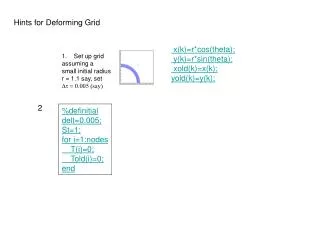
Hints for Deforming Grid x(k)=r*cos(theta); y(k)=r*sin(theta); xold(k)=x(k); yold(k)=y(k); • Set up grid • assuming a • small initial radius • r = 1.1 say, set • Dt = 0.005 (say) 2 %definitial delt=0.005; St=1; for i=1:nodes T(i)=0; Told(i)=0; end
Iteration in a time step (Between 20 and 50) Calculate and store coefficients for k=1:loopcount k1=sup(i,k); k2=sup(i,k+1); xL(1) = x(i); %xL=local x-coordinate xL(2) = x(k1); xL(3) = x(k2); yL(1) = y(i); %yL=local y-coordinate yL(2) = y(k1); yL(3) = y(k2); xLold(1) = xold(i); xLold(2) = xold(k1); xLold(3) = xold(k2); yLold(1) = yold(i); yLold(2) = yold(k1); yLold(3) = yold(k2); %grid velocity contributions vxL(1)=(xL(1)-xLold(1))/delt; vxL(2)=(xL(2)-xLold(2))/delt; vxL(3)=(xL(3)-xLold(3))/delt; vyL(1)=(yL(1)-yLold(1))/delt; vyL(2)=(yL(2)-yLold(2))/delt; vyL(3)=(yL(3)-yLold(3))/delt; %CV Volunme v=xLold(2)*yLold(3)-xLold(3)*yLold(2)-xLold(1)*yLold(3)... +xLold(1)*yLold(2)+yLold(1)*xLold(3)-yLold(1)*xLold(2)/2; Volpold(i)=Volpold(i)+v/3;
%Diffusion Contributions Face 1 ap(i) = ap(i) - Nx(1) * dely + Ny(1) * delx; apdis(i)=apdis(i)-Nx(1) * dely + Ny(1) * delx; a(i,k) = a(i,k) + Nx(2) * dely - Ny(2) * delx; adis(i,k) = adis(i,k) + Nx(2) * dely - Ny(2) * delx; a(i,k+1) = a(i,k+1) + Nx(3) * dely - Ny(3) * delx; adis(i,k+1) = adis(i,k+1) + Nx(3) * dely - Ny(3) * delx; %GRID ADVECTION CONTRIBUTION CENTRAL DIFF vxf=(5*vxL(1)+5*vxL(2)+2*vxL(3))/12; vyf=(5*vyL(1)+5*vyL(2)+2*vyL(3))/12; vxf=(5*vxL(1)+5*vxL(2)+2*vxL(3))/12; vyf=(5*vyL(1)+5*vyL(2)+2*vyL(3))/12; qf=vxf*dely-vyf*delx; ap(i)= ap(i) +St*((5/12)*qf+(2/12)*qf); a(i,k) = a(i,k) + St*((5/12)*qf); a(i,k+1)=a(i,k+1)+St*(2/12)*qf);
%SET BOUNDARY FOR Temp for i=1:nodes BC(i)=0; %coefficient part BB(i)=0; %constant part end for k=1:n_b(4) BC(B(4,k))=1e18; BB(B(4,k))=1e18; end for k=1:n_b(2) BC(B2,k))=1e18; end %code for Transient for i=1:nodes apt(i)=St*Volpold(i)/delt; end
%Solve for T for iter=1:50 for i= 1:nodes RHS=apt(i)*Told(i)+BB(i); for k=1:n_s(i) RHS=RHS+a(i,k)*T(sup(i,k)); end T(i)=RHS/(apt(i)+ap(i)+BC(i)); end end
Adjust Points on melt Front for k=1:n_b(2) %global boundary point index point=B(2,k); %signed length if k==1 delx=(x(B(2,k+1))-x(B(2,k)))/2; dely=(y(B(2,k+1))-y(B(2,k)))/2; end if k>1 & k < n_b(2) delx=(x(B(2,k+1))-x(B(2,k-1)))/2; dely=(y(B(2,k+1))-y(B(2,k-1)))/2; end if k==n_b(2) delx=(x(B(2,k))-x(B(2,k-1)))/2; dely=(y(B(2,k))-y(B(2,k-1)))/2; end %Heat flow into volue around boundary point RHS=0; for i=1:n_s(point) RHS=RHS+a(point,i)*T(S(point,i)); end c=-delx/(dely+1e-6); if k==1 c=1e-6; end if k==n_b(2) c=1e6; end if abs(c)<abs(1.0/c) adjx(point)=delt*RHS/(dely-c*delx); adjy(point)=c*adjx(point); else adjy(point)=delt*RHS/((1.0/c)*dely-delx); adjx(point)=(1.0/c)*adjy(point); end end i Dy Dx
%Adjust x positions of Nodes for i=1:nodes BC(i)=0; %coeficient part BB(i)=0; %constant part end for k=1:n_b(3) BC(B(3,k))=1e18; end for k=1:n_b(3) BC(B(2,k))=1e18; BB(B(2,k))=1e18*adjx(B(2,k)); end for k=1:n_b(4)(4) BC(B(4,k))=1e18; end Calculate and store coefficients for iter=1:50 for i= 1:nodes RHS=BB(i); for k=1:n_s(i) RHS=RHS+adis(i,k)*adjx(sup(i,k)); end adjx(i)=RHS/(apdis(i)+BC(i)); end end Similar for y adjust in BUT take care to identify boundaries %defupdate for i=1:nodes x(i)=x(i)+0.4*(xold(i)+adjx(i)-x(i)); y(i)=y(i)+0.4*(yold(i)+adjy(i)-y(i)); end END OF ITS GO BACK TO Calculate and store coefficients
After 20-50 its Finish Time step Before next time step swap old for new %oldnew for i=1:nodes xold(i)=x(i); yold(i)=y(i); Told(i)=T(i); r(i)=sqrt(x(i)^2+y(i)^2); end