Simulation Analysis and Random Number Generation
DADSS. Simulation Analysis and Random Number Generation. Administrative Details. Homework 6 due Homework 7 due next Monday Very interesting DADSS-like talk taking place tomorrow at noon in the Moot Board Room. Rema Padman

Simulation Analysis and Random Number Generation
E N D
Presentation Transcript
DADSS Simulation Analysis and Random Number Generation
Administrative Details • Homework 6 due • Homework 7 due next Monday • Very interesting DADSS-like talk taking place tomorrow at noon in the Moot Board Room. • Rema Padman • Come! If 5/7 of you come, I’ll include an additional “free” problem on Exam 2
Question • Profit projections • Units sold ~ N(100K,10K) • Unit Price ~ N(25, 6) • Fixed cost = 1mil • Variable cost = N(7.5,7.5) or 2, whichever is greater
What is Simulation? • “A mathematical model that is studied by means of simulation” • Question: Why? • To “simulate” is to replicate or copy the process of something • Many mathematical models are so complicated that it is impossible or impractical to “solve” them via a closed-form or analytic solution
Analytical vs Computational • An example: d = r × t • What happens to distance traveled if I double my speed? • If we want to study the behavior of distance, we have a simple mathematical model with which to do that • Sensitivity of distance with respect to the rate • Sensitivity of distance with respect to the time • Both • Because this model is simple, we can develop an explicit understanding analytically
Analytical vs Computational • Another example: A check-out line in a supermarket • What happens to the amount of time I spend in line if the supermarket opens another register? • Even if we could set out a system of equations that represented this situation (“queueing theory”), it would be very difficult to analyze analytically • Instead, we can analyze the actual problem by building a simulation (or replica) of the problem and studying that • The difference? Control • We get to “experiment”
Possible Future States • Simulation models are useful primarily for allowing examination of what could happen or what could have happened • Two roles for simulation analysis: • Studying uncertainty • Think of a decision tree with 100,000+ of branches • Studying complex systems • Systems for which an analytical representation is impractical or impossible
Simulation Analysis in General • Describe the problem • As always: Choices, States, Acts, Consequences • Create a model of the problem • The role of abstraction • If your simulation model is as complicated as the real thing, why use it? • Provide a characterization of any uncertainty • “Run” the model as many times as necessary to develop an understanding of the system
Building Blocks • Random Numbers • Confidence Intervals • Probability Distributions • Dependence Relationships • Iteration (generally, a “computational mechanism”)
Random Numbers in Theory • What is a random number? • First, note that we can represent any real number just by looking at the range [0,1] • Real number between 0 and 100? • Multiply 100 by RAND() • Real number between -50 and 50? • Multiply 100 by RAND() and subtract 50 • Real number between a and b? • Multiply RAND() by (b - a) and add to a • Only concerned with uniform random numbers between 0 and 1 • everything else can be obtained from uniform [0,1] random numbers • Characteristics of uniform random numbers • Unpredictable • Evenly distributed
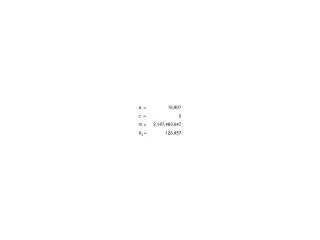
Random Numbers in Practice • In Excel: RAND() produces a number that is uniformly distributed between 0 and 1 • That is, each number in that interval is equally likely • True Randomness vs Pseudorandomness • Cycle period (in Excel 1013 random numbers before a cycle) • Prior to Excel 2003, Excel’s cycle used to be 1 million (106)
Using Random Numbers • Back to the coin toss problem • A simple simulation model • Toss a coin until you see one of the following sequences: • HHT: You win $10 • THH: You lose $10 • A coin toss is a random process, so we should be able to build a simulation model to examine this problem • IF(RAND()<0.5,“H”,“T”) • Spreadsheet will be on Blackboard
Coin Toss Results • Solving the coin toss problem by hand, it’s very clear that the answer is that HHT wins 25% of the time and THH wins 75% of the time • However, even running the simulation for 100 iterations doesn’t produce exactly that number as an average result • Simulation models converge on the true solution -- but that true solution is often a limit result (i.e., assuming an infinite number of iterations)
Convergence • In the coin toss example, if we added more runs of the simulation model, our mean answer would get more accurate • The range around it would get tighter • We refer to this process as convergence, and the width of the range around the estimated mean is a confidence interval
Convergence: An Example • Roll a 6-sided die 10 times • How many rolls out of the 10 will result in an even number being thrown?
Convergence: An Example • Roll a 6-sided die 10 times • How many rolls out of the 10 will result in an even number being thrown?
Convergence: An Example • Roll a 6-sided die 10 times • How many rolls out of the 10 will result in an even number being thrown?
The Central Limit Theorem • Convergence is a consequence of the Central Limit Theorem • Simple version: Averages are distributed normally (for all distributions with finite moments) • Consequence: Once we calculate the average of a set of simulation runs, we then know exactly what the uncertainty around that estimated average is because we can calculate the confidence interval
The Central Limit Theorem • 95% Confidence Interval • ALWAYS provide confidence intervals!!! • Convergence is a function of , the square root of the number of runs of the simulation, under most conditions
Speed of Convergence • Although the CLT guarantees convergence, it doesn’t say how quickly it might arrive – it’s a limit property, after all • Often, convergence takes very long – especially for very complicated problems • Convergence occurs on the order of the inverse of the square root of n – the denominator in the confidence interval equation • Can we do better? What about 1/n?
Random Numbers – Without the Randomness • Quasirandom Numbers (“low discrepancy sequences”) • Stratification is what improves convergence, not necessarily randomness • Is randomness critical to the analysis?
Quasirandom Numbers • How they work is beyond the scope of this class (it involves number theory) • In general, they are designed to be “self-avoiding” or “space-filling” • By removing randomness completely, you can often obtain better stratification • Variance reduction methods • Latin Hypercube sampling in @Risk • Control Variate Methods • Antithetic Variables Methods • Common Random Numbers • An example to experiment with: Richtmyer numbers (one of the earliest QR sequences)
Imperative! • Simulation is more about doing than about saying! • You must “get your hands dirty” to truly understand this material. • Use the models on Blackboard; build your own • We cannot possibly cover every Excel/@Risk function in class – you will need to explore on your own

