In-Flight Calibration for PN Camera Analysis at Ringberg, April 2-4, 2002
430 likes | 462 Vues
Detailed analysis of 110 sources with energy ranges from 0.3 keV to 10.0 keV using King model profile. Investigation includes building radial profile, fitting curves, and 2-D modeling for PSF.

In-Flight Calibration for PN Camera Analysis at Ringberg, April 2-4, 2002
E N D
Presentation Transcript
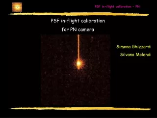
PSF in-flight calibration for PN camera Simona Ghizzardi Silvano Molendi Ringberg, April 2-4, 2002
DATA SAMPLE: - 110 SOURCES (TARGET) included ENERGY RANGES: 0.3 keV [200-400] eV 0.6 keV [400-800] eV 1.0 keV [800-1200] eV 1.8 keV [1200-2400] eV 3.7 keV [2400-5000] eV 6.5 keV [5000-8000] eV 10.0 keV [8000-12000] eV OFF-AXIS ANGLES: from on-axis position up to ~10 arcmin - most of them are observed within ~ 2 arcmin. Ringberg, April 2-4, 2002
Analysis procedure and PSF model We adopt the same procedure and the same algorithm used for the two MOS cameras. The pixel size of the PSF images is taken 1.1” . According to the MOS results, the profile of the PSF is well represented by a King model: PSF = KING + BKG Ringberg, April 2-4, 2002
King profile core slope Two shape parameters: core radius (rc) and slope (a) IT CAN BE INTEGRATED ANALYTICALLY IN rdr!!! Ringberg, April 2-4, 2002
Building the radial profile • We merged the observations having • the same source target • the same pointing position • different filters and/or operating mode ---> • ---> different pile-up levels • The centroid is determined accounting for the mask of the detector • For each curve a good fitting range must be defined (points suffering • for pile-up must be excluded). Ringberg, April 2-4, 2002
We bin the image (with larger bins at larger radii) RADIAL PROFILE: dN/dA (the area is not 2pr dr because of the mask) each (squared) pixel is assigned to the (round) bin to which its CENTER belongs for these pixels it works fairly these pixels belong to two different bins in comparable fractions the effect is less important at larger radii Algorithm for the averaged radial profile • Energy selection and pattern (0-12) selection • BASIC METHOD ADDITIONAL RECIPE ADDED TO THE BASIC PROCEDURE We enclose each pixel in a circle. If the circle is fully enclosed in the bin then the pixel is too. If the circle is partly enclosed in another bin, the pixel may belong to two bins: we divide such pixels in NSUBPIXELS Ringberg, April 2-4, 2002
The physical pixel size is 4.1”, not much smaller than the core radius of the PSF. The calibration of the core is quite tricky The frame time is smaller than the MOS one. The pile-up effect is less important The effective area is larger than the MOS one. Good statistics Ringberg, April 2-4, 2002
Fitting the radial profiles In order to enhance the statistics, we fit simultaneously the different curves with different pile-up levels PSF = King + BKG a e rc are the same for each curve BKG and the normalization are different for each curve for each energy and off-axis angle we derive a and rc. Ringberg, April 2-4, 2002
2-D FIT: rc = rc(E, J) a = a(E, J) SLOPE: IT HAS A ROUGHLY CONSTANT BEHAVIOR EVEN IF THE 2-D BEST FIT DECREASES FOR OFF-AXIS ANGLES INCREASING. CORE: THE LINEAR DECREASING BEHAVIOR IS NOT WELL REPRESENTED BY THE 2-D FIT. 0.3 keV THE 2-D FIT IS DRIVEN BY THE ON-AXIS POINTS. Ringberg, April 2-4, 2002
2-D FIT: rc = rc(E, J) a = a(E, J) SLOPE: IT HAS A ROUGHLY CONSTANT BEHAVIOR EVEN IF THE 2-D BEST FIT DECREASES FOR OFF-AXIS ANGLES INCREASING. CORE: THE LINEAR DECREASING BEHAVIOR IS NOT WELL REPRESENTED BY THE 2-D FIT. 0.6 keV THE 2-D FIT IS DRIVEN BY THE ON-AXIS POINTS. Ringberg, April 2-4, 2002
2-D FIT: rc = rc(E, J) a = a(E, J) SLOPE: IT HAS A ROUGHLY CONSTANT BEHAVIOR EVEN IF THE 2-D BEST FIT DECREASES FOR OFF-AXIS ANGLES INCREASING. CORE: THE LINEAR DECREASING BEHAVIOR IS NOT WELL REPRESENTED BY THE 2-D FIT. 1.0 keV THE 2-D FIT IS DRIVEN BY THE ON-AXIS POINTS. Ringberg, April 2-4, 2002
2-D FIT: rc = rc(E, J) a = a(E, J) SLOPE: IT HAS A ROUGHLY CONSTANT BEHAVIOR EVEN IF THE 2-D BEST FIT DECREASES FOR OFF-AXIS ANGLES INCREASING. CORE: THE LINEAR DECREASING BEHAVIOR IS NOT WELL REPRESENTED BY THE 2-D FIT. 1.8 keV THE 2-D FIT IS DRIVEN BY THE ON-AXIS POINTS. Ringberg, April 2-4, 2002
2-D FIT: rc = rc(E, J) a = a(E, J) SLOPE: IT HAS A ROUGHLY CONSTANT BEHAVIOR EVEN IF THE 2-D BEST FIT DECREASES FOR OFF-AXIS ANGLES INCREASING. CORE: THE LINEAR DECREASING BEHAVIOR IS NOT WELL REPRESENTED BY THE 2-D FIT. 3.7 keV THE 2-D FIT IS DRIVEN BY THE ON-AXIS POINTS. Ringberg, April 2-4, 2002
2-D FIT: rc = rc(E, J) a = a(E, J) SLOPE: IT HAS A ROUGHLY CONSTANT BEHAVIOR EVEN IF THE 2-D BEST FIT DECREASES FOR OFF-AXIS ANGLES INCREASING. CORE: THE LINEAR DECREASING BEHAVIOR IS NOT WELL REPRESENTED BY THE 2-D FIT. 6.5 keV THE 2-D FIT IS DRIVEN BY THE ON-AXIS POINTS. Ringberg, April 2-4, 2002
2-D FIT: rc = rc(E, J) a = a(E, J) SLOPE: IT HAS A ROUGHLY CONSTANT BEHAVIOR EVEN IF THE 2-D BEST FIT DECREASES FOR OFF-AXIS ANGLES INCREASING. CORE: THE LINEAR DECREASING BEHAVIOR IS NOT WELL REPRESENTED BY THE 2-D FIT. 10. keV THE 2-D FIT IS DRIVEN BY THE ON-AXIS POINTS. Ringberg, April 2-4, 2002
2-D FIT: rc = rc(E, J) a = a(E, J) SLOPE: IT HAS A ROUGHLY CONSTANT BEHAVIOR EVEN IF THE 2-D BEST FIT DECREASES FOR OFF-AXIS ANGLES INCREASING. CORE: THE LINEAR DECREASING BEHAVIOR IS NOT WELL REPRESENTED BY THE 2-D FIT. 1.0 keV THE 2-D FIT IS DRIVEN BY THE ON-AXIS POINTS. Ringberg, April 2-4, 2002
2-D FIT: rc = rc(E, J) a = a(E, J) SLOPE: IT HAS A ROUGHLY CONSTANT BEHAVIOR EVEN IF THE 2-D BEST FIT DECREASES FOR OFF-AXIS ANGLES INCREASING. CORE: THE LINEAR DECREASING BEHAVIOR IS NOT WELL REPRESENTED BY THE 2-D FIT. 1.8 keV THE 2-D FIT IS DRIVEN BY THE ON-AXIS POINTS. Ringberg, April 2-4, 2002
2-D FIT: rc = rc(E, J) a = a(E, J) SLOPE: IT HAS A ROUGHLY CONSTANT BEHAVIOR EVEN IF THE 2-D BEST FIT DECREASES FOR OFF-AXIS ANGLES INCREASING. CORE: THE LINEAR DECREASING BEHAVIOR IS NOT WELL REPRESENTED BY THE 2-D FIT. 3.7 keV THE 2-D FIT IS DRIVEN BY THE ON-AXIS POINTS. Ringberg, April 2-4, 2002
BINNING Data are not well represented by the 2-D data because they present a very large scatter. The 2-D fit ( but also each 1-D fit for any fixed energy) is completely driven by the on-axis data. We bin on the off-axis angle variable with bin 12” wide. Ringberg, April 2-4, 2002
2-D FIT: rc = rc(E, J) a = a(E, J) BINS for off axis angle: 12” SLOPE: IT HAS A ROUGHLY CONSTANT BEHAVIOR CORE: IT LINEARLY DECREASES FOR INCREASING OFF AXIS ANGLES 0.3 keV Ringberg, April 2-4, 2002
2-D FIT: rc = rc(E, J) a = a(E, J) BINS for off axis angle: 12” SLOPE: IT HAS A ROUGHLY CONSTANT BEHAVIOR CORE: IT LINEARLY DECREASES FOR INCREASING OFF AXIS ANGLES 0.6 keV Ringberg, April 2-4, 2002
2-D FIT: rc = rc(E, J) a = a(E, J) BINS for off axis angle: 12” SLOPE: IT HAS A ROUGHLY CONSTANT BEHAVIOR CORE: IT LINEARLY DECREASES FOR INCREASING OFF AXIS ANGLES 1.0 keV Ringberg, April 2-4, 2002
2-D FIT: rc = rc(E, J) a = a(E, J) BINS for off axis angle: 12” SLOPE: IT HAS A ROUGHLY CONSTANT BEHAVIOR CORE: IT LINEARLY DECREASES FOR INCREASING OFF AXIS ANGLES 1.8 keV Ringberg, April 2-4, 2002
2-D FIT: rc = rc(E, J) a = a(E, J) BINS for off axis angle: 12” SLOPE: IT HAS A ROUGHLY CONSTANT BEHAVIOR CORE: IT LINEARLY DECREASES FOR INCREASING OFF AXIS ANGLES 3.7 keV Ringberg, April 2-4, 2002
2-D FIT: rc = rc(E, J) a = a(E, J) BINS for off axis angle: 12” SLOPE: IT HAS A ROUGHLY CONSTANT BEHAVIOR CORE: IT LINEARLY DECREASES FOR INCREASING OFF AXIS ANGLES 6.5 keV Ringberg, April 2-4, 2002
2-D FIT: rc = rc(E, J) a = a(E, J) BINS for off axis angle: 12” SLOPE: IT HAS A ROUGHLY CONSTANT BEHAVIOR CORE: IT LINEARLY DECREASES FOR INCREASING OFF AXIS ANGLES 10. keV Ringberg, April 2-4, 2002
2-D FIT: rc = rc(E, J) a = a(E, J) BINS for off axis angle: 12” SLOPE: IT HAS A ROUGHLY CONSTANT BEHAVIOR CORE: IT LINEARLY DECREASES FOR INCREASING OFF AXIS ANGLES 1.0 keV Ringberg, April 2-4, 2002
2-D FIT: rc = rc(E, J) a = a(E, J) BINS for off axis angle: 12” SLOPE: IT HAS A ROUGHLY CONSTANT BEHAVIOR CORE: IT LINEARLY DECREASES FOR INCREASING OFF AXIS ANGLES 1.8 keV Ringberg, April 2-4, 2002
2-D FIT: rc = rc(E, J) a = a(E, J) BINS for off axis angle: 12” SLOPE: IT HAS A ROUGHLY CONSTANT BEHAVIOR CORE: IT LINEARLY DECREASES FOR INCREASING OFF AXIS ANGLES 3.7 keV Ringberg, April 2-4, 2002
Profiles using the best fit values Ringberg, April 2-4, 2002
Profiles using the best fit values Ringberg, April 2-4, 2002
WHY SUCH A SCATTER ? Out of time events can affect the slope of the profile Pile up is less evident in the PN data. Are we neglecting a pile up effect? Centroiding is very difficult because of the large size of the pixels. This makes the determination of the core uncertain especially for the Small Window op. mode. …TO BE INVESTIGATED Ringberg, April 2-4, 2002
FULL FRAME SMALL WINDOW Ringberg, April 2-4, 2002
WHY SUCH A SCATTER ? Out of time events can affect the slope of the profile Pile up is less evident in the PN data. Are we neglecting a pile up effect? Centroiding is very difficult because of the large size of the pixels. This makes the determination of the core uncertain especially for the Small Window op. mode. …TO BE INVESTIGATED Ringberg, April 2-4, 2002
WHY SUCH A SCATTER ? Out of time events can affect the slope of the profile Pile up is less evident in the PN data. Are we neglecting a pile up effect? Centroiding is very difficult because of the large size of the pixels. This makes the determination of the core uncertain especially for the Small Window op. mode. …TO BE INVESTIGATED Ringberg, April 2-4, 2002
King Core Radius for PN Ringberg, April 2-4, 2002
King Slope for PN Ringberg, April 2-4, 2002
BEST FIT VALUES Ringberg, April 2-4, 2002
ENCIRCLED ENERGY FRACTION Ringberg, April 2-4, 2002
Range of Application Ringberg, April 2-4, 2002
CONCLUSIONS By using a large set of data we modeled the PSF profile with a King function and provided the best fit values of the core and of the slope as functions of the energy and of the off-axis angle. To be done … We must include in the sample some other off-axis sources to enlarge the region of the range of application. Check on : evaluation of the background in the Small Window measures out of time events pile-up centroiding procedures in order to reduce the scatter of the points Ringberg, April 2-4, 2002