Understanding RMSE: Differences Between Actual and Predicted Values in Regression Analysis
This chapter explores the intricacies of regression analysis, particularly focusing on the concept of Root Mean Square Error (RMSE) and its computation. It explains the difference between actual and predicted values, detailing how RMSE quantifies this difference and serves as a measure of prediction accuracy. The chapter also discusses residual plots and the implications of patterns within them, highlighting the significance of normal distribution approximations and homoscedasticity. Key statistical principles, including the correlation coefficient and its relationship with RMSE, are examined to enhance understanding.

Understanding RMSE: Differences Between Actual and Predicted Values in Regression Analysis
E N D
Presentation Transcript
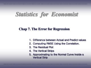
Chap 7. The Error for Regression Difference between Actual and Predict values Computing RMSE Using the Correlation. The Residual Plot The Vertical Strips Approximating to the Normal Curve Inside a Vertical Strip
1 2 3 4 5 Computing RMSE Using the Correlation The Residual Plot The Vertical Strips INDEX Difference between Actual and Predict Values Approximating to the Normal Curve Inside a Vertical Strip
1. Difference between Actual and Predict Values Root-Mean-Square-Error (RMSE) Error Actual value Root-Mean-Square Error (RMSE) Standard Error of Estimate Standard Error of Regression 회귀직선 Estimate
1. Difference between Actual and Predict Values Estimation error1 Korean men 4514 with age 10-90 - Average height = 167.5cm - SD of height = 8.5cm - Average weight = 63.5kg - SD of weight = 11.9kg - Correlation coefficient = 0.67 height141cm. average weight of height 141cm is 38.7kg residual = actual weight – predicted weight = 54.5kg – 38.7kg = +15.8kg Residual of A Residual of B 67.4kg – 84.0kg = -16.6kg
1. Difference between Actual and Predict Values Estimation error 2 • Estimation error • actual weight – predicted weight • generally called, residual. • The overall size of these errors in measured by taking their root mean square. weight error Vertical distance from the line actual predicted height
1. Difference between Actual and Predict Values Computing the RMSE meaning • A typical point on a scatter plot is above or below the regression line by 8.9kg. (vertical distance) The divisor • degrees of freedom = 4514-2 = 4512 • Computing the errors are based on the regression line. • The regression line is defined by slope and intercept (lowering the • degree of freedom)
1. Difference between Actual and Predict Values Regression line & RMSE vs. Average & SD The Normal curve. Following 68-95 rule. Group average height of the regression line Distance from the center(RMSE)
2RMSE 1RMSE regression 2RMSE 1RMSE regression 95% 68% 1. Difference between Actual and Predict Values Regression and rule of thumb About 68% of the points on a scatter diagram will be within 1RMSE of the regression line; about 95% of them will be within 2RMSE.
y residual= (actual y) – (average y) actual estimate = (average y) x 1. Difference between Actual and Predict Values Elementary method for RMSE Estimate y ignoring x → a horizontal line for estimates. This elementary RMSE is SDy.
1 2 3 4 5 Computing RMSE Using the Correlation The Residual Plot The Vertical Strips INDEX Difference between Actual and Predict Values Approximating to the Normal Curve Inside a Vertical Strip
y y Regression lines SDy RMSE Average y x x 2. Computing RMSE Using the Correlation RMSE of the regression line and SDy RMSE of regression is about r = 1 → RMSE = 0 r = -1 → RMSE = 0 r = 0 → RMSE SDy Degrees of freedom RMSE of regression < SDy because the regression line get closer to the points than the horizontal line. ref: Regression line is for ‘much closer to the more scatters’.
2. Computing RMSE Using the Correlation RMSE and Correlation coefficient RMSE Measures vertically spread around the regression line in absolute y-terms. Correlation coefficient Measures spread relative to the SD without units. We can get the RMSE from SDy using the correlation coefficient..
2. Computing RMSE Using the Correlation Regression analysis and correlation coefficient • r describes the clustering of the points around the SD line, relative to the SDs • Associated with each 1SD increase in x there is an increase of only r SDs in y, on the average • r determines the accuracy of the regression predictions, through the formula RMSE = SDy . • RMSE describes how the regression line summarize data well.
1 2 3 4 5 Computing RMSE Using the Correlation The Residual Plot The Vertical Strips INDEX Difference between Actual and Predict Values Approximating to the Normal Curve Inside a Vertical Strip
3. The Residual Plot Plotting the Residual Plot • The residuals average out to 0. • The regression line for the residual plot is horizontal x-axis. The reason is that all the trend up or down has been taken out of the residual, and is in the residuals.
3. The Residual Plot A residual with a strong pattern The residual plot should not have a strong pattern. With a mistake to use a regression line, such a pattern appears.
1 2 3 4 5 Computing RMSE Using the Correlation The Residual Plot The Vertical Strips INDEX Difference between Actual and Predict Values Approximating to the Normal Curve Inside a Vertical Strip
35 40 45 50 55 60 65 70 75 80 85 90 95 100 4. The Vertical Strips Scatter plot and histogram inside the vertical strips Group with height about 170 cm people Group with height about 165cm people The two histograms have similar shapes, and their SDs are nearly the same.
4. The Vertical Strips Homoscedasticity and Heteroscedasticity Homoscedasticity Heteroscedasticity All the vertical strips in a scatter plot show similar amounts of spread and the SDs of weight are not related to x-value. The size of it is about RMSE. The SDs of income in groups vary to the vertical strips.In this case, the RMSE of the regression line only gives a sort of average error across all the different x-values.
1 2 3 4 5 Computing RMSE Using the Correlation The Residual Plot The Vertical Strips INDEX Difference between Actual and Predict Values Approximating to the Normal Curve Inside a Vertical Strip
Approximating to the Normal Curve inside a Vertical Strip Impossible to approximate Estimates are meaningless themselves , The errors does not follow normal curve. <heteroscedastic> <nonlinear> The regression method uwing RMSE is off by different amounts in different parts of the scatter plot.
Approximating to the Normal Curve inside a Vertical Strip example1 Ex) Midterm and final scores of econometrics in spring semester year 2002 midterm average = 27.9 midterm SD = 8.5 final average = 56.4 final SD = 13.8 r = 0.49 an oval shaped scatter plot. (1) What percentage of students got 66 or over on the final? (2) What percentage of students whose midterm score is 33 got 66 or over on the final?
Approximating to the Normal Curve inside a Vertical Strip example 1 • Even Midterm related statistics or correlation coefficient are not necessary. ☞ By standard normal curve, 24% ☞ z=0.7
Approximating to the Normal Curve inside a Vertical Strip example 1 (2) We get new average using the regression analysis, new SD from RMSE of regression line. 1. Midterm score is above the average by 0.6 SDx. 2. r= 0.49; 0.60.49 = 0.3 3. Final score is above by 0.3 SDy = 4.1 4. New average is 56.4 + 4.1 = 60.5 . Regression Analysis Method z = 0.5 By standard normal curve, 31 %