Download
1 / 24
240 likes | 300 Vues
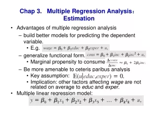
Chap 3. Multiple Regression Analysis : Estimation. Advantages of multiple regression analysis build better models for predicting the dependent variable. E.g. generalize functional form. Marginal propensity to consume Be more amenable to ceteris paribus analysis Key assumption:

E N D
Chap 3. Multiple Regression Analysis:Estimation • Advantages of multiple regression analysis • build better models for predicting the dependent variable. • E.g. • generalize functional form. • Marginal propensity to consume • Be more amenable to ceteris paribus analysis • Key assumption: • Implication: other factors affecting wage are not related on average to educ and exper. • Multiple linear regression model:
OLS Estimator • OLS: Minimize • ceteris paribus interpretations: • Holding fixed, then • Thus, we have controlled for the variables when estimating the effect of x1 on y.
Holding Other Factors Fixed • The power of multiple regression analysis is that it provides this ceteris paribus interpretation even though the data have notbeen collected in a ceteris paribus fashion. • it allows us to do in non-experimental environments what natural scientists are able to do in a controlled laboratory setting: keep other factors fixed.
OLS and Ceteris Paribus Effects • measures the effect of x1 on y after x2,…, xkhave been partialled or netted out. • Two special cases in which the simple regression of y on x1will produce the same OLS estimate on x1as the regression of y on x1and x2. --The partial effect of x2 on y is zero in the sample. That is, -- x1and x2 are uncorrelated in the sample. --Example
data1: 1832 rural household reg consum laborage reg consum laborage financialK corr laborage financialK reg consum laborage reg consum laborage laboredu corr laborage laboredu
Goodness-of-fit • R-sq also equal the squared correlation coef. between the actual and the fitted values of y. • R-sq never decreases, and it usually increases when another independent variable is added to a regression. • The factor that should determine whether an explanatory variable belongs in a model is whether the explanatory variable has a nonzero partial effect on y in the population.
The Expectation of OLS Estimator • Assumption 1-4 • Linear in parameters • Random sampling • Zero conditional mean • No perfect co-linearity • none of the independent variables is constant; • and there are no exact linear relationships among the independent variables • Theorem (Unbiasedness) • Under the four assumptions above, we have:
Notice 1: Zero conditional mean • Exogenous Endogenous • Misspecification of function form (Chap 9) • Omitting the quadratic term • The level or log of variable • Omitting important factors that correlated with any independent v. • Measurement Error (Chap 15, IV) • Simultaneously determining one or more x-s with y (Chap 16) • Try to use exogenous variable! (Geography, History)
Omitted Variable Bias: The Simple Case • Omitted Variable Bias • The true population model: • The underspecified OLS line: • The expectation of : (46) 前面3.2节中是x1对x2回归
The expectation of , where the slope coefficient from the regression of x2 on x1, so then, Only two cases where is unbiased, , x2 does not appear in the true model; , x2 and x1 are uncorrelated in the sample; 前面3.2节中是x1对x2回归
Notice 2: No Perfect Collinearity • An assumption only about x-s, nothing about the relationship between u and x-s • Assumption MLR.4 does allow the independent variables to be correlated; they just cannot be perfectly correlated • If we did not allow for any correlation among the independent variables, then multiple regression would not be very useful for econometric analysis • How to deal with collinearity problem? Drop correlated variable, respectively. (corr=0.7)
Notice 3: Over-Specification • Inclusion of an irrelevant variable: • does not affect the unbiasedness of the OLS estimators. • including irrelevant variables can have undesirable effects on the variances of the OLS estimators.
Variance of The OLS Estimators • Assumption 5 • Homoskedasticity: • Gauss-Markov Assumptions (for cross-sectional regression): Assumption 1-5 • Linear in parameters • Random sampling • Zero conditional mean • No perfect co-linearity • Homoskedasticity
Theorem (Sampling variance of OLS estimators) • Under the five assumptions above:
More about • The statistical properties of y on x=(x1, x2, …, xk) • Error variance • only one way to reduce the error variance: to add more explanatory variables — not always possible and desirable (multi-collinearity) • The total sample variations in xj: SSTj • Increase the sample size
Multi-collinearity • The linear relationships among the independent v-s. • 其他解释变量对xj的拟合优度(含截距项) • If k=2: • :the proportion of the total variation in xjthat can be explained by the other independent variables High (but not perfect) correlation between two or more of the in dependent variables is called multicollinearity.
Small sample size Small sample size Low SSTj • one thing is clear: everything else being equal, for estimating , it is better to have less correlation between xj and the other V-s.
Notice: The influence of multi-collinearity • A high degree of correlation between certain independent variables can be irrelevant as to how well we can estimate other parameters in the model. • x2和x3之间的高相关性并不直接影响x1的回归系数的方差,极端的情形就是X1和x2、x3都不相关。同时前面我们知道,增加一个变量并不会改变无偏性。在多重共线性的情形下,估计仍然无偏,我们关心的变量系数的方差也与其他变量之间的共线性没有直接关系,尽管方差会变化,只要t值仍然显著,共线性不是大问题。 • How to “solve” the multi-collinearity? • Dropping some v.? 如果删除了总体模型中的一个变量,则可能会导致内生性。 参见注释
Estimating : Standard Errors of the OLS Estimators df=number of observations-number of estimated parameters Theorem 3.3Unbiased estimation of Under the Gauss-Markov Assumption, MLR 1-5, 参见注释
While the presence of heteroskydasticity does not cause bias in the , it does lead to bias in the usual formula for , which when then invalidates the standard errors. This is important because any regression package compute 3.58 as the default standard error for each coefficient.
Gauss-Markov Assumptions (for cross-sectional regression): • 1. Linear in parameters • 2. Random sampling • 3. Zero conditional mean • 4. No perfect co-linearity • 5. Homoskedasticity • 违反1-4中的任何一个假设将导致有偏的回归系数; • 违反假设5不会导致有偏估计,但是会导致对回归系数标准差的计算出现偏差,从而影响对回归系数的显著性的统计推断; • 多元回归中的其他几个问题: • 6. 异方差问题: 无法计算回归系数的标准差 • 7. 小样本问题: SST 小,方差非最小 • 8. 多重共线性问题: Rj-sq大,方差非最小
Efficiency of OLS: The Gauss-Markov Theorem • BLUEs • Best: smallest variance • Linear • Unbiased • Estimator 定理的含义: 1. 无需寻找其他线性组合的无偏估计量; 2. 如果G-M假设有一个不成立,则BLUE不成立。
Implications • Theory and right functional form • Include the variables necessary, do not miss them, especially those included in existing literature!! • Get a good measure of the variables • Use exogenous variables