Reliability Analysis & Cost Modeling
Reliability Analysis & Cost Modeling. with your host…. Dave Hy, the rocket scientist guy. (Not to be confused with the untalented and scientifically-challenged Bill Nye, the stupid guy). 426 Lecture #9 Reliability Analysis and Cost Modeling Readings: L&W Section 19.2 L&W Chapter 20


Reliability Analysis & Cost Modeling
E N D
Presentation Transcript
Reliability Analysis & Cost Modeling with your host…. Dave Hy, the rocket scientist guy (Not to be confused with the untalented and scientifically-challenged Bill Nye, the stupid guy)
426 Lecture #9 Reliability Analysis and Cost Modeling Readings: L&W Section 19.2 L&W Chapter 20 L&W Chapter 22 Reliability = The science of forestalling failure Why is this needed? Ans.: The vulnerability and inaccessibility of space systems (Things have to be kept working right on their own)
Penalty for lack of reliability: Economic Loss = How much a failure costs “Reliability of components or systems” = the probability that they will not fail. Reliability analysis uses the laws of probability. Probability has two meanings: Relative frequency interpretation “State of knowledge” (Laplace) Pr(A) 0 Sure that A won’t happen 0.5 Don’t know one way or the other 1.0 A is certain to happen
Probability – What you need to know Suppose: Pr[A] = Probability that event “A” will happen Then: Pr[Not A] = 1 - Pr[A] If A and B are independent: Pr[A and B] = Pr[A]Pr[B] If Fs = system failure probability, then: VF = Expected cost of failure= FsVs (Vs = economic resources needed to compensate for the loss of the s/c and its launch)
Using these simple facts, we can address: Given the reliability of components, the reliability of the system How to estimate component reliability How to maximize reliability cost-effectively
4. Approach sequence 1. Orbit plane change burn 2. transfer burn 9. Grappling completed 3. Debris orbit insertion 5. Prox Ops system enabled 7. Grappling system enabled 8. Non-bouncing contact 6. Low velocity approach R4= 0.98 R1= 0.99 R2= 0.98 R3= 0.99 R9= 0.99 R8= 0.99 R6= 0.98 R7= 0.99 R5= 0.95 Successful attachment Given the reliability of components, find the reliability of a subsystem Example: Rendezvous, and attachment to a debris object (Rk = probability of success for component “k”)
Let RRAS denote the probability that the Rendezvous and Attachment System works. Because each of the 9 components has to work: RRAS = Pr{ Component 1 works and Component 2 works and … …Component 9 works} We can assume in this case that the success of each component is independent of all the others – RAS success is compounded of independent events. Therefore: RRAS = Pr{ Component 1 works} x Pr{Component 2 works} x… Pr{Component 9 works} = R1 x R2 x R3 x R4 x R5 x R6 x R7 x R8 x R9 = (0.99) (0.98) (0.99) (0.98) (0.95) (0.99) (0.98) (0.99) (0.99) = 0.850 Finally, the probability of failure, FRAS, is: FRAS = 1- RRAS = 1-0.850 = 0.15 Note: Despite just a few percent failure probability for each component, the failure probability for the whole RAS builds up to 15%
Methods to reduce Fs ±Fault avoidance: Use design margins, high quality parts, close inspection and testing, etc. “Do it right the first time” ΔFault tolerance:Design in the ability to operate after the failure of some components. ΩFunctional redundancy:After failure of a component, another component performs the functions of the failed unit, even though its primary function is something different. πGround support robustnessThe vehicle allows ground support to perform “workarounds” to solve problems (frequently involves software manipulations)
Fly by remote control subsystem 1. Orbit plane change burn 2. Hohmann transfer burn 9. Grappling completed 3. Debris orbit insertion 6. Low velocity approach 8. Non-bouncing contact 4. Approach sequence 7. Grappling system enabled R4= 0.98 R1= 0.99 R2= 0.98 R3= 0.99 R7= 0.98 R8= 0.99 R9= 0.99 R6= 0.99 R5.A= 0.95 R5.B= 0.95 5.A Telerobotic system enabled 5.B Prox Ops system enabled Methods to reduce Fs – Example of Functional Redundacy Successful attachment
R5.A= 0.95 R5.B= 0.95 5.Atelerobotic system enabled 5.BProx Ops system enabled To calculate reliability, first concentrateon the “Fly by remote control” block: When we have components in parallel, the whole block works if any one of the components works. To find the reliability in such cases, first find the probability of failure – call it FRobust control Clearly, the whole block can’t fail unless all the components fail: FRobustcontrol = Pr{ Component 5.A fails and Component 5.B fails} But the failure of each component is independent of the other component, so: FRobustcontrol = Pr{ Component 5.A fails}x Pr{Component 5.B fails} But the probability of Component 5.A failing is 1-R5.A, etc. FRobustcontrol = (1-R5.A)( 1-R5.B) = (0.05)x(0.05) = 0.0025 Now, the reliability of this block, call it RRobustcontrol is just: RRobustcontrol = 1 - FRobustcontrol = 0.9975
Note: By meansof redundancy,we’ve decreasedthe likelihood of failure in the closeapproach control from 5% to 0.25%. To finish up our calculation ofreliability for the new (partially redundant) subsystem, justcompute RRASas before, but substitute RRobustcontrol in place of R5: RLRA = R1 x R2 x R3xR4 x RRobustcontrol xR6 x R7 x R8 x R9 = (0.99) (0.98) (0.99)(0.98) (0.9975) (0.99) (0.98) (0.99) (0.99) = 0.893 So,we’veraised the overall reliability by over 4% ____________________________________________________________
Note: When you have a calculation such as R1 x R2 x R3 x R4 x R5 x R6 xR7 x R8 x R9, where there are many factors and each component reliability is close to unity, you can get a quick (but good) approximation by simply subtracting the sum of the failure probabilities from unity; REDL = R1 x R2 x R3 x R4 x R5 x R6 x R7 x R8 x R9 = (1 – F1) (1 – F2) …(1 – F9) = 1 – (F1+ F2+… +F9) + products of small numbers ≈ 1 – (F1+ F2+… +F9) … which is a lot simpler (and less prone to roundoff error)than multiplying many numbers, each one very slightly less than 1.0. (In the present case, the approximation gives RCDS ≈ 0.888) _______________________________________________
Cost concepts showing optimum reliability budget [Hecht, 1973]. F0 is the probability of failure for the baseline system. (From L&W, 2nd Edition)
Cost Estimation Process • (L&W Chapter 20) • ×First compose a WBS (Work Breakdown Structure), using Fig. 20-2 as a model÷L&W distinguish three life cycle phases:>Research, Development, Test & Evaluation (RDT&E) =Production Theoretical First Unit (TFU) <Operations and Maintenance (O&M) • We emphasize here : RDT&E and TFU. • RDT&E as understood in thecontext of L&W includes the development of reasonably mature technology elements up to the level required for the flight. It does not refer to the basic technology development and flight validation demos.
Cost Estimating Methods 1)Detailed, bottom-up estimating 2)Analogy-based estimating (find a similar item then try to adjust for differences) 3)Parametric estimating. Use math relations between design parameters and cost that are compiled from statistics of previous programs. These relations are called “CERs” (Cost Estimating Relationships) For preliminary design, (3) is best. But (3) is subject to caveats: CER’s only applicable to the range of historical data Parametric estimating not satisfactory for estimating items involving major technological advancements or fundamental paradigm shifts. (see L&W, p.788)
Recommended Process First, use (3) for initial estimates Then revisit system elements that are new or innovative and use method (2) (or even (1)) For the new and innovative elements, we will request detailed “bottom up” data on similar items from NASA
For the Parametric estimating stage, take the following steps: A) Use Table 20-6 (for small sats.)*, combined with Table 20-9 (that breaks out the fractions due to nonrecurring costs versus recurring costs, to give the RDT&E versus TFU costs) B) Apply the factors given in Table 20-8 to the RDT&E CERs to allow for development heritage. C) Compute software costs using Table 20-10 D) Next estimate ground segment and operations costs using Table 20-11
E)Communications equipment: Table 20-13 F)Launch costs: Table 20-14 G)Finally, be sure to apply the inflation factors relative to the year 2000 in Table 20-1. ______________________ * We use CERs for small sat.s because, although the statistical data base is smaller, it pertains to programs wherein consistent efforts were made to reduce costs
Cost-Risk AnalysisMLE = “Most likely estimate” = mean value of cost SE = “Standard Error” = The standard deviation about the mean Cost risk due to uncertainties arising from technical innovations are estimated by the “Technology readiness level” (TRL) – a graduated scale introduced by NASA For this project, we need to produce two main outputs: 1)Costs for RDT&E and for the TFU, with uncertainty estimates.2)Identify the basically new technologies that will be needed to implement the design and estimate their (relatively low) TRLs.
Considerations for the design work: Basic Objectives (Definition of “Mission Success”), Probability Calculations and How You Do the Mission Are All Completely Entwined
“Knee of the curve” Best possible mission outcome Performance Uncertainty Mission Benefit Cost Uncertainty Expenditure, $. So your mission is to maximize all these probabilities while minimizing the cost of each component
At long last………… The End has arrived