Download
1 / 38
380 likes | 413 Vues
Explore data visualization, descriptive statistics, and distribution analysis in psychology. Learn to interpret graphs and tables to describe center, spread, and shape of data.

E N D
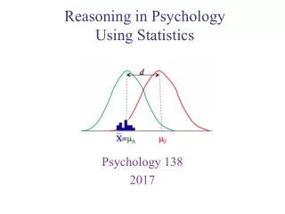
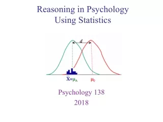
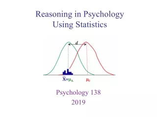
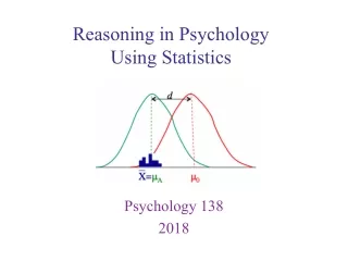
Reasoning in PsychologyUsing Statistics Psychology 138 2017
Let’s collect set of data • I’ll pass out some pairs of dice • Collect n=36 data points • 12 people roll a pair of dice three times Type numbers here: Rolling the dice
Distribution • The distribution of a variable is a summary of all the different values of a variable • The set of all of the outcomes of rolling the dice • Both type (each value) and token (each instance) • Un-organized, the overall pattern and properties of the distribution are difficult to see • A “picture” of the distribution is usually helpful Type numbers here: Distributions David McCandless: The beauty of data visualization
Descriptive statistics • Statistical tools/procedures to help organize, summarize, and simplify large sets of data (distributions) • Important descriptive properties of distribution • Center • Where most of the data in the distribution are • Spread (variability) • How similar/dissimilar are the scores in the distribution? • Shape • Symmetric vs. asymmetric (skew) • Unimodal vs. multimodal Describing Distributions
Today’s focus Describing Distributions
A “picture” of the distribution is usually helpful • Gives a good sense of the properties of the distribution • Many different ways to display distribution • Table • Frequency distribution table • Stem and leaf plot • Graphs Describing Distributions
A “picture” of the distribution is usually helpful • Gives a good sense of the properties of the distribution • Many different ways to display distribution • Table • Frequency distribution table • Stem and leaf plot • Graphs Describing Distributions
The values of the variable The proportion of tokens at each value The percentage of tokens at each value The number of tokens of each variable Cumulative percentage p = f/N N=total Frequency distribution table
10% got a 1 or worse Quiz: “What % got this score or worse?” 10 Cumulative percent
15% got a 2 & 10% got a 1 25% got a 2 or worse Quiz: “What % got this score or worse?” 25 10 Cumulative percent
10% got a 3 & 15% got a 2 & 10% got a 1 35% got a 3 or worse Quiz: “What % got this score or worse?” 35 25 10 Cumulative percent
35% got a 4 & 10% got a 3 & 15% got a 2 & 10% got a 1 70% got a 4 or worse Quiz: “What % got this score or worse?” 70 35 25 10 Cumulative percent
20% got a 5 & 35% got a 4 & 10% got a 3 & 15% got a 2 & 10% got a 1 90% got a 5 or worse Quiz: “What % got this score or worse?” 90 70 35 25 10 Cumulative percent
10% got a 6 & 20% got a 5 & 35% got a 4 & 10% got a 3 & 15% got a 2 & 10% got a 1 100% got a 6 or worse Quiz: “What % got this score or worse?” 100 90 70 35 25 10 Cumulative percent
Fill in numbers from our class: Sample distribution n = 36 Frequency distribution: sum of 2 dice
Value D1+D2 Value D1+D2 Value D1+D2 D2 D2 D2 D1 D1 D1 frequency frequency frequency 1 1 4 12 7 4 11 7 2 2 11 4 7 6 10 3 7 3 3 10 3 7 2 10 7 9 6 9 4 6 9 5 6 9 6 8 6 8 5 5 8 5 4 8 5 8 5 Total outcomes = 62 = 36 = 1+2+3+4+5+6+5+4+3+2+1 = 36 Theoretical Frequency distribution: sum of 2 dice
p = probability when predicting p = proportion when describing what you observed Think of this as defining our population distribution of the outcome of tossing two dice Total outcomes = 62 = 36 = 1+2+3+4+5+6+5+4+3+2+1 = 36 Theoretical Frequency distribution: sum of 2 dice
population sample Sampling error Theoretical frequency distribution & class sample(Actual fs are from a previous term.)
Important properties of distribution • Center • Where most of the data in the distribution are • Spread (variability) • How similar/dissimilar are the scores in the distribution? • Shape • Symmetric vs. asymmetric (skew) • Unimodal vs. multimodal Distributions
7 What is the most frequent score? Describing the distribution
Two-thirds of the data are here What is the most frequent score? Where do most of the scores lie? Describing the distribution
Maximum score: 12 Minimum score: 2 What is the most frequent score? Where do most of the scores lie? What was the range of scores? Describing the distribution
A “picture” of the distribution is usually helpful • Gives a good sense of the properties of the distribution • Many different ways to display distribution • Table • Frequency distribution table • Stem and leaf plot • Graphs Distributions
10 9 8 7 6 5 4 • Distribution of exam scores (section 01): • 67, 90, 92, 58, 76, 75, 84, 92, 78, 93, 89, 74, 62, 98, 75, 73, 75, 89, 89, 76, 65, 49 0 2 2 3 8 4 9 9 9 6 5 8 4 5 3 5 6 7 2 5 8 9 Stem and Leaf Plots
0 10 5 3 0 9 0 2 2 3 8 9 4 3 8 4 9 9 9 5 4 3 3 2 2 1 1 0 7 3 4 5 5 5 6 6 8 6 5 5 2 2 6 2 5 7 8 5 8 2 4 9 • Distribution of exam scores (section 01): • 67, 90, 92, 58, 76, 75, 84, 92, 78, 93, 89, 74, 62, 98, 75, 73, 75, 89, 89, 76, 65, 49 • Distribution of exam scores (section 03): • 72, 90, 83, 58, 66, 65, 84, 95, 72, 93, 89, 70, 42, 100, 71, 73, 75, 62, 62, 74, 65 Stem and Leaf Plots
A “picture” of the distribution is usually helpful • Gives a good sense of the properties of the distribution • Many different ways to display distribution • Table • Frequency distribution table • Stem and leaf plot • Graphs • Graphs types • Continuous variable: • histogram, line graph (frequency polygons) • Categorical (discrete) variable: • pie chart, bar chart Distributions
Histogram • Line graph Graphs for continuous variables
Bar chart • Pie chart Graphs for categorical variables
Important properties of distribution • Center • Where most of the data in the distribution are • Spread (variability) • How similar/dissimilar are the scores in the distribution? • Shape • Symmetric vs. asymmetric (skew) • Unimodal vs. multimodal Distributions
tail tail • Symmetric • Asymmetric Positive Skew Negative Skew Shape
Major mode Minor mode • Unimodal (one mode) • Multimodal • Bimodal examples Shape
Coming up in future lectures: • In addition to pictures of the distribution, numerical summaries are also presented. • Numeric Descriptive Statistics • Shape • Skew (symmetry) & Kurtosis (shape) • Number of modes • Measures of Center • Measures of Variability (Spread) • In lab, create basic tables and graphs both by hand and using SPSS • If time in lecture there are some SPSS show and tell slides Descriptive statistics
Drag & drop Drag & drop SPSS: Bar graph
Drag & drop Drag & drop SPSS: Cluster bar graph
Legend SPSS: Cluster bar graph
Drag & drop Drag & drop SPSS: Histogram