Download
1 / 67
680 likes | 893 Vues
دانشگاه صنعتي اميرکبير ( پلي تکنيک تهران). Estimation of the Intrinsic Dimension. Nonlinear Dimensionality Reduction , John A. Lee, Michel Verleysen, Chapter3. Overview. Introduce the concept of intrinsic dimension along with several techniques that can estimate it

E N D
دانشگاه صنعتي اميرکبير (پلي تکنيک تهران) Estimation of the Intrinsic Dimension Nonlinear Dimensionality Reduction , John A. Lee, Michel Verleysen, Chapter3
Overview • Introduce the concept of intrinsic dimension along with several techniques that can estimate it • Estimators based on fractal geometry • Estimators related to PCA • Trail and error approach
q-dimension (Cont.) • The support of μ is covered with a (multidimensional) grid of cubes with edge lengthε. • Let N(ε) be the number of cubes that intersect the support of μ. • let the natural measures of these cubes be p1, p2, . . . , pN(ε). • pi may be seen as the probability that these cubes are populated
q-dimension (Cont.) • For q ≥ 0, q ≠ 1, these limits do not depend on the choice of the –grid, and give the same values
Capacity dimension • Setting q equal to zero • In this definition, dcapdoes not depend on the natural measures pi • dcap is also known as the ‘box-counting’ dimension
Capacity dimension (Cont.) • When the manifold is not known analytically and only a few data points are available, the capacity dimension is quite easy to estimate:
Intuitive interpretation of the capacity dimension • Assuming a three-dimensional space divided in small cubic boxes with a fixed edge lengthℇ • The number of occupied boxes grows • For a growing one-dimensional object, proportionally to the object length • for a growing two-dimensional object, proportionally to the object surface. • for a growing three-dimensional object, proportionally to the object volume. • Generalizing to a P-dimensional object like a P-manifold embedded in RD
Correlation dimension • Where q = 2 • The term correlation refers to the fact that the probabilities or natural measures pi are squared.
Correlation dimension (Cont.) • C2(ε) is the number of neighboring points lying closer than a certain threshold ε. • This number grows as a length for a 1D object, as a surface for a 2D object, as a volume for a 3D object, and so forth.
Correlation Dim.(Cont.) • When the manifold or fractal object is only known by a countable set of points
Practical estimation • When knowledge is finite number of points • Capacity and correlation dimensions • However for each situation calculating limit to zero is impossible in practice
the slope of the curve is almost constant between 1 ≈ exp(−6) = 0.0025 and 2 ≈ exp(0) = 1
Dimension estimators based on PCA • The model of PCA is linear • The Estimator works only for manifolds containing linear dependencies (linear subspaces) • For more complex manifolds, PCA gives at best an estimate of the global dimensionality of an object.(2D for spiral manifold, Macroscopic effect)
Local Methods • Decomposing the space into small patches, or “space windows” • Ex. Nonlinear generalization of PCA • 1. Windows are determined by clustering the data (Vector quantization) • 2. PCA is carried out locally, on each space Window • 3. Compute weighted average on localities
The fraction of the total variance spanned by the first principal component of each cluster or space window. The corresponding dimensionality (computed by piecewise linear interpolation) for three variance fractions (0.97, 0.98, and0.99)
Properties • The dimension given by local PCA is scale-dependent, like the correlation dimension. • Low number of space windows-> Large window-> Macroscopic structure of spiral (2D) • Optimum window -> small pieces of spiral (1D) • High number of space windows-> too small window-> Noise scale(2D)
Propeties • local PCA requires more data samples to yield an accurate estimate(dividing the manifold into non overlapping patches.) • PCA is repeated for many different numbers of space windows, then the computation time grows.
Trial and error • 1. For a manifold embedded in a D-dimensional space, reduce dimensionality successively to P=1,2,..,D. • 2. Plot Ecodec as a function of P. • 3. Choose a threshold, and determine the lowest value of P such that Ecodec goes below it (An elbow).
Additional refinement • Using statistical estimation methods like cross validation or bootstrapping: • Ecodecis computed by dimensionality reduction on several subsets that are randomly drawn from the available data. • This results in a better estimation of the reconstruction errors, and therefore in a more faithful estimation of the dimensionality at the elbow. • Huge computational requirements.
ComparisionsData Set • 10D data set • Intrinsic Dim : 3 • 100, 1000, and 10,000 observations • White Gaussian noise, with std 0.01
PCA estimator • Number of observations does not greatly influence the results • Nonlinear dependences hidden in the data sets
Correlation Dimension Much more sensitive to the number of available observations.
the correlation dimension is much • slower than PCA but yields higher quality results Edge effects appear: the dimensionality is slightly underestimated The noise dimensionality appears more clearly as the number of observations grows. The correlation dimension is much slower than PCA but yields higher quality results
Local PCA estimator The nonlinear shape of the underlying manifold for large windows
Local PCA estimator (cont.) too small window , rare samples PCA is no longer reliable, because the windows do not contain enough points.
Local PCA estimator (cont.) • Local PCA yields the right dimensionality. • The largest three normalized eigen values remain high for any number of windows, while the fourth and subsequent ones are negligible. • It is noteworthy that for a single window the result of local PCA is trivially the same as for PCA applied globally, But as the number of windows is increasing, the fourth normalized eigen value is decreasing slowly. • Local PCA is obviously much slower than global PCA, but still faster than the correlation dimension
Trial and error • The number of points does not play an important role. • The DR method slightlyover estimates the dimensionality. • Although the method relies on a nonlinear model, the manifold may still be too curved to achieve a perfect embedding in a space having the same dimension as the exact manifold dimensionality. • The overestimation observed for PCA does not disappear but is only attenuated when switching to an NLDR method.
Concluding remarks • PCA applied globally on the whole data set remains the simplest and fastest one. • Its results are not very convincing: the dimension is almost always overestimated if data do not perfectly fit the PCA model. • Method relying on a nonlinear model is very slow. • The overestimation that was observed with PCA does not disappear totally.
Concluding remarks • Local PCA runs fast if the number of windows does not sweep a wide interval. • local PCA has given the right dimensionality for the studied data sets. • The correlation dimension clearly appears as the best method to estimate the intrinsic dimensionality. • It is not the fastest of the four methods, but its results are the best and most detailed ones, giving the dimension on all scales.
دانشگاه صنعتي اميرکبير (پلي تکنيک تهران) Distance Preservation Nonlinear Dimensionality Reduction , John A. Lee, Michel Verleysen, Chapter4
The motivation behind distance preservation is that any manifold can be fully described by pairwise distances. • Presrving geometrical structure
Outline • Metric space & most common distance measures • Metric Multi dimensional scaling • Geodesic and graph distances • Non linear DR methods
Spatial distancesMetric space • A space Y with a distance function d(a, b) between two points a, b ∈ Y is said to be a metric space if the distance function respects the following axioms: • Nondegeneracy d(a, b) = 0 if and only if a = b. • Triangular inequality d(a, b) ≤ d(c, a) + d(c, b). • Nonnegativity. • Symmetry
In the usual Cartesian vector space RD, the most-used distance functions are derived from the Minkowski norm • Dominance distance (p = ∞) • Manhattan distance (p=1) • Euclidean distance(p = 2) • Mahalanobis distance • A straight generalization of the Euclidean distance
Metric Multi dimensional scaling • Classical metric MDS is not a true distance preserving method. • Metric MDS preserves pairwise scalar products instead of pairwise distances(both are closely related). • Is not a nonlinear DR. • Instead of pairwise distances we can use pairwise “similarities”. • When the distances are Euclidean MDS is equivalent to PCA.
Metric MDS • Generative model • Where components of x are independent or uncorrelated • W is a D-by-p matrix such that • Scalar product between observations Gram matrix Both Y and X are unknown; only the matrix of pairwise scalar products S,Gram matrix, is given.
Metric MDS (Cont.) • Eigen value decomposition of Gram matrix • P-dimensional latent variables • Criterion of metric MDS
Metric MDS (Cont.) • Metric MDS and PCA give the same solution. • When data consist of distances or similarities prevent us from applying PCA -> Metric MDS. • When the coordinates are known, PCA spends fewer memory resources than MDS. • ??
Geodesic distance • Assuming that very short Euclidean distances are preserved • Euclidean longer distances are considerably stretched. • Measuring the distance along the manifold and not through the embedding space
Geodesic distance • Distance along a manifold • In the case of a one-dimensional manifold M, which depends on a single latent variable x
Geodesic distance (Cont.) • The integral then has to be minimized over all possible paths that connect the starting and ending points. • Such a minimization is intractable since it is a functional minimization. • Anyway, the parametric equations of M(and P) are unknown; only some (noisy) points of M are available.
Graph dist. • Lack of analytical information -> reformulation of problem. • Minimizing an arc length between two points on a manifold. • Minimize the length of a path (i.e., a broken line). • The path should be constrained to follow the underlying manifold. • In order to obtain a good approximationof the true arc length, a fine discretizationof the manifold is needed. • Only the smallest jumps will be permitted. (K-rule,ε-rule )
Graph dist. • ``
Graph dist. • How to compute the shortest paths in a weighted graph? Dijkstra • It is proved that the graph distance approximates the true geodesic distance in an appropriate way.
Isomap • Isomap is a NLDR method that uses the graph distance as an approximation of the geodesic distance. • Isomap inherits one of the major shortcomings of MDS: a very rigid model. • If the distances in D are not Euclidean, Implicitly assumed that the replacement metric yields distances that are equal to Euclidean distances measured in some transformed hyperplane.