Describing Location in a Distribution: Percentiles, Cumulative Frequency Graphs, and z-scores
310 likes | 345 Vues
Learn how to measure position using percentiles, interpret cumulative relative frequency graphs, use z-scores for comparison, and describe density curves in data distributions. Explore examples with baseball wins, test scores, and income distributions.

Describing Location in a Distribution: Percentiles, Cumulative Frequency Graphs, and z-scores
E N D
Presentation Transcript
Chapter 2: Modeling Distributions of Data Section 2.1 Describing Location in a Distribution The Practice of Statistics, 4th edition - For AP* STARNES, YATES, MOORE
Chapter 2Modeling Distributions of Data • 2.1Describing Location in a Distribution • 2.2Normal Distributions
Section 2.1Describing Location in a Distribution Learning Objectives After this section, you should be able to… • MEASURE position using percentiles • INTERPRET cumulative relative frequency graphs • MEASURE position using z-scores • TRANSFORM data • DEFINE and DESCRIBE density curves
WARM UP 25 32 15 19 20 22 24 30 • Find the quartiles of the data. • What percentage of the data is to the left of Q1? • What percentage of the data is to the right of Q2?
WARM UP 25 32 15 19 20 22 24 30 1. Find the quartiles of the data. Q1 = 19.5, Q2 = 23 and Q3 = 27.5 2. What percentage of the data is to the left of Q1? 25% 3. What percentage of the data is to the right of Q2? 50%
Describing Location in a Distribution • Measuring Position: Percentiles • One way to describe the location of a value in a distribution is to tell what percent of observations are less than it. Definition: The pth percentile of a distribution is the value with p percent of the observations less than it. Example, p. 85 Jenny earned a score of 86 on her test. How did she perform relative to the rest of the class? 6 7 7 2334 7 5777899 8 00123334 8 569 9 03 6 7 7 2334 7 5777899 8 00123334 8 569 9 03 Her score was greater than 21 of the 25 observations. Since 21 of the 25, or 84%, of the scores are below hers, Jenny is at the 84th percentile in the class’s test score distribution.
Example • Example: Wins in Major League Baseball • The stemplot below shows the number of wins for each of the 30 Major League Baseball teams in 2009. • Calculate and interpret the percentiles for the Colorado Rockies who had 92 wins, the New York Yankees who had 103 wins, and the Cleveland Indians who had 65 wins. Key: 5|9 represents a team with 59 wins.
Describing Location in a Distribution • Cumulative Relative Frequency Cumulative Relative Frequency adds the counts in the frequency column for the current class and all previous classes. Example: Let’s look at the frequency table for the ages of the 1st 44 US presidents when they were inaugurated.
Describing Location in a Distribution • Cumulative Relative Frequency Graphs A cumulative relative frequency graph displays the cumulative relative frequency of each class of a frequency distribution.
Interpreting Cumulative Relative Frequency Graphs Describing Location in a Distribution Use the graph from page 88 to answer the following questions. • Was Barack Obama, who was inaugurated at age 47, unusually young? • Estimate and interpret the 65th percentile of the distribution 65 11 58 47
Example • Example: State Median Household Incomes • Here is a cumulative relative frequency graph showing the distribution of median household incomes for the 50 states and the District of Columbia. The point (50, 0.49) means that 49% of the states had a median household income of less than $50,000. a) California, with a median household income of $57,445, is at what percentile? Interpret this value. b) What is the 25th percentile for this distribution? What is another name for this value?
Describing Location in a Distribution • Measuring Position: z-Scores • A z-score is a value that tells us how many standard deviations from the mean an observation falls, and in what direction. Definition: If x is an observation from a distribution that has known mean and standard deviation, the standardized value of x is: A standardized value is often called a z-score. Example: Jenny earned a score of 86 on her test. The class mean is 80 and the standard deviation is 6.07. What is her standardized score?
Describing Location in a Distribution • Using z-scores for Comparison We can use z-scores to compare the position of individuals in different distributions. The single-season home run record for major league baseball has been set just three times since Babe Ruth hit 60 home runs in 1927. Roger Maris hit 61 in 1961, Mark McGwire hit 70 in 1998 and Barry Bonds hit 73 in 2001. In an absolute sense, Barry Bonds had the best performance of these four players, since he hit the most home runs in a single season. However, in a relative sense this may not be true. To make a fair comparison, we should see how these performances rate relative to others hitters during the same year. Calculate the standardized score for each player and compare.
Example • The single-season home run record for major league baseball has been set just three times since Babe Ruth hit 60 home runs in 1927. Roger Maris hit 61 in 1961, Mark McGwire hit 70 in 1998 and Barry Bonds hit 73 in 2001. In an absolute sense, Barry Bonds had the best performance of these four players, since he hit the most home runs in a single season. However, in a relative sense this may not be true. To make a fair comparison, we should see how these performances rate relative to others hitters during the same year. Calculate the standardized score for each player and compare. • Ruth: 60 – 7.2 = 5.44 McGwire: 70 – 20.7 = 3.87 9.7 12.7 • Maris: 61 – 18.8 = 3.16 Bonds: 73 – 21.4 = 3.91 13.4 13.2 Although all 4 performances were outstanding, Babe Ruth can still lay claim to being the single-season home run champ, relatively speaking.
WARM UP Mrs. Navard measured the heights of all her Statistics students in inches. She found that their mean was 67 with a standard deviation of 4.29. • 1. Lynette, a student in the class, is 65 inches tall. Find and interpret her z-score. • 2. Another student in the class, Brent, is 74 inches tall. How tall is Brent compared with the rest of the class? • 3. Brent is a member of the school’s basketball team. The mean height of the players is 76 inches. If Brent’s height translates to a z-score of -0.85, what is the standard deviation of the team member’s heights?
Answers • Mrs. Navard measured the heights of all her Statistics students in inches. She found that their mean was 67 with a standard deviation of 4.29. • 1. Lynette, a student in the class, is 65 inches tall. Find and interpret her z-score. z = -0.47 ; Lynette’s height is 0.47 standard deviations below the mean • 2. Another student in the class, Brent, is 74 inches tall. How tall is Brent compared with the rest of the class? • Brent’s z-score is 1.63. He is about 1.63 standard deviations above the mean. • 3. Brent is a member of the school’s basketball team. The mean height of the players is 76 inches. If Brent’s height translates to a z-score of -0.85, what is the standard deviation of the team member’s heights? 2.35 inches
Z-Scores Practice 1. A normal distribution of scores has a standard deviation of 10. Find the z-scores corresponding to each of the following values: a. A score of 60, where the mean score of the sample data values is 40. b. A score that is 30 points below the mean. c. A score of 80, where the mean score of the sample data values is 30. d. A score of 20, where the mean score of the sample data values is 50.
Z-Scores Practice 2. IQ scores have a mean of 100 and a standard deviation of 16. Albert Einstein reportedly had an IQ of 160. a. What is the difference between Einstein’s IQ and the mean? b. How many standard deviations is that? c. If we consider “usual IQ scores to be those that convert z scores between -2 and 2, is Einstein’s IQ usual or unusual?
Z-Scores Practice 3. Women’s heights have a mean of 63.6 in. and a standard deviation of 2.5 inches. Find the z-score corresponding to a woman with a height of 70 inches and determine whether the height is unusual.
Z-Scores Practice 4. Three students take equivalent stress tests. Which is the highest relative score? a. A score of 144 on a test with a mean of 128 and a standard deviation of 34. b. A score of 90 on a test with a mean of 86 and a standard deviation of 18. c. A score of 18 on a test with a mean of 15 and a standard deviation of 5.
Describing Location in a Distribution • Transforming Data Transforming converts the original observations from the original units of measurements to another scale. Transformations can affect the shape, center, and spread of a distribution. Effect of Adding (or Subracting) a Constant • Adding the same number a (either positive, zero, or negative) to each observation: • adds a to measures of center and location (mean, median, quartiles, percentiles), but • Does not change the shape of the distribution or measures of spread (range, IQR, standard deviation).
Example • Example: Here is a graph and table of summary statistics for a sample of 30 test scores. The maximum possible score on the test was a 50. • Suppose that the teacher is nice and wants to add 5 points to each test score. How would this affect the shape, center and spread of the data?
Example • The measures of center and position (mean, median, quartiles, and percentiles) all increased by 5. However, the shape and spread (range, IQR, standard deviation) of the distribution did not change.
Describing Location in a Distribution • Transforming Data Effect of Multiplying (or Dividing) by a Constant • Multiplying (or dividing) each observation by the same number b (positive, negative, or zero): • multiplies (divides) measures of center and location by b • multiplies (divides) measures of spread by |b|, but • does not change the shape of the distribution Example: Suppose that the teacher wants to convert each test score to percents. Since the test was out of 50 points, he should just multiply each score by 2 to make them out of 100. How would this change the shape, center and spread of the data? The measures of center, location and spread will all double. However, even though the distribution is more spread out, the shape will not change!!!
WARM UP In 1995 the Educational Testing Service (ETS) adjusted the scores of SAT tests. Before ETS re-centered the SAT verbal test, the mean of all test scores was 450. 1. How would adding 50 points to each score affect the mean? 2. The standard deviation was 100 points. What would the standard deviation be after adding 50 points? 3. The times in the men’s combined event at the Winter Olympics are reported in minutes and seconds. The mean and standard deviation of the slalom times are 94.27 and 5.28 respectively. Suppose instead that we report the times in minutes. What would the resulting mean and standard deviation be?
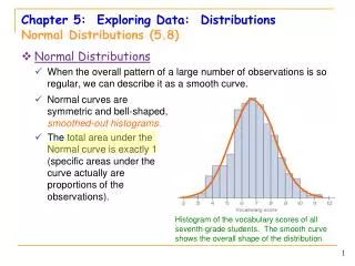
Describing Location in a Distribution • Density Curves • In Chapter 1, we developed a kit of graphical and numerical tools for describing distributions. Now, we’ll add one more step to the strategy. • So far our strategy for exploring data is : • 1. Graph the data to get an idea of the overall pattern • 2. Calculate an appropriate numerical summary to describe the center and spread of the distribution. Sometimes the overall pattern of a large number of observations is so regular, that we can describe it by a smooth curve, called a density curve.
Describing Location in a Distribution • Density Curve • Definition: • A density curve is a curve that • is always on or above the horizontal axis, and • has area exactly 1 underneath it. • A density curve describes the overall pattern of a distribution. The area under the curve and above any interval of values on the horizontal axis is the proportion of all observations that fall in that interval. The overall pattern of this histogram of the scores of all 947 seventh-grade students in Gary, Indiana, on the vocabulary part of the Iowa Test of Basic Skills (ITBS) can be described by a smooth curve drawn through the tops of the bars.
Density Curves • NOTE: No real set of data is described by a density curve. It is simply an approximation that is easy to use and accurate enough for practical use. • Describing Density Curves • The median of the density curve is the “equal-areas” point. • The mean of the density curve is the “balance” point.
Section 2.1Describing Location in a Distribution Summary In this section, we learned that… • There are two ways of describing an individual’s location within a distribution – the percentile and z-score. • A cumulative relative frequency graph allows us to examine location within a distribution. • It is common to transform data, especially when changing units of measurement. Transforming data can affect the shape, center, and spread of a distribution. • We can sometimes describe the overall pattern of a distribution by a density curve (an idealized description of a distribution that smooths out the irregularities in the actual data).
Looking Ahead… In the next Section… • We’ll learn about one particularly important class of density curves – the Normal Distributions • We’ll learn • The 68-95-99.7 Rule • The Standard Normal Distribution • Normal Distribution Calculations, and • Assessing Normality