Problems

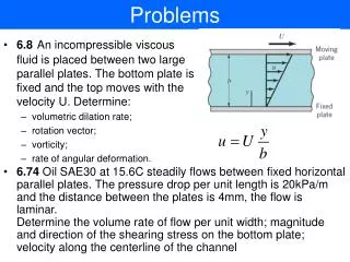
1. Problems • 6.8An incompressible viscous fluid is placed between two large parallel plates. The bottom plate is fixed and the top moves with the velocity U. Determine: • volumetric dilation rate; • rotation vector; • vorticity; • rate of angular deformation. • 6.74 Oil SAE30 at 15.6C steadily flows between fixed horizontal parallel plates. The pressure drop per unit length is 20kPa/m and the distance between the plates is 4mm, the flow is laminar.Determine the volume rate of flow per unit width; magnitude and direction of the shearing stress on the bottom plate; velocity along the centerline of the channel

2. Problems • 7.19. One type of viscosimeter is designed as shown in the figure. The reservoir is filled with liquid and the time required for the liquid to drop from Hi to Hf determined. Obtain relationship between viscosity m and draining time t. Assume the variables involved Hi,Hf, D and specific weight g. • 7.50 The drag D=f(d,D,V,r). What dimensional parameters will be used? If in experiment d=5mm, D=12.5mm and V=0.6m/s, the drag is 6.7x10-3N. Estimate drag on a sphere in 0.6 m diam tube where water flowing with a velocity of 1.8 m/s and the diameter of sphere is such that the similarity is maintained

3. Viscous flow in pipes

4. General characteristic of Pipe flow • pipe is completely filled with water • main driving force is usually a pressure gradient along the pipe, though gravity might be important as well open-channel flow Pipe flow

5. Laminar or Turbulent flow well defined streakline, one velocity component velocity along the pipe is unsteady and accompanied by random component normal to pipe axis

6. Laminar or Turbulent flow • In this experiment water flows through a clear pipe with increasing speed. Dye is injected through a small diameter tube at the left portion of the screen. Initially, at low speed (Re <2100) the flow is laminar and the dye stream is stationary. As the speed (Re) increases, the transitional regime occurs and the dye stream becomes wavy (unsteady, oscillatory laminar flow). At still higher speeds (Re>4000) the flow becomes turbulent and the dye stream is dispersed randomly throughout the flow.

7. Entrance region and fully developed flow • fluid typically enters pipe with nearly uniform velocity • the length of entrance region depends on the Reynolds number dimensionless entrance length

8. Pressure and shear stress no acceleration, viscous forces balanced by pressure pressure balanced byviscous forces and acceleration

9. Fully developed laminar flow • we will derive equation for fully developed laminar flow in pipe using 3 approaches: • from 2nd Newton law directly applied • from Navier-Stokes equation • from dimensional analysis

10. 2nd Newton’s law directly applied

11. 2nd Newton’s law directly applied doesn’t depend on radius

12. 2nd Newton’s law directly applied for Newtonian liquid: Flow rate:

13. 2nd Newton’s law directly applied • if gravity is present, it can be added to the pressure:

14. Navier-Stokes equation applied • The assumptions and the result are exactly the same as Navier-Stokes equation is drawn from 2nd Newton law in cylindrical coordinates:

15. Dimensional analysis applied assuming pressure drop proportional to the length:

16. Turbulent flow • in turbulent flow the axial component of velocity fluctuates randomly, components perpendicular to the flow axis appear • heat and mass transfer are enhanced in turbulent flow • in many cases reasonable results on turbulent flow can be obtained using Bernoulli equation (Re=inf).

17. Fluctuation in turbulent flow • All parameters fluctuate in turbulent flow (velocity, pressure, shear stress, temperature etc.) behave chaotically • flow parameters can be described as an average value + fluctuations (random vortices) • can be characterized by turbulence intensity and time scale of fluctuation turbulence intensity

18. Shear stress in turbulent flow • Turbulent flow can often be thought of as a series of random, 3-dimensional eddy motions (swirls) ranging from large eddies down through very small eddies • Vortices transfer momentum, so the shear force is higher compared with laminar flow:

19. Shear stress in turbulent flow • The turbulent nature of the flow of soup being stirred in a bowl is made visible by use of small reflective flakes that align with the motion. The initial stirring causes considerable small and large scale turbulence. As time goes by, the smaller eddies dissipate, leaving the larger scale eddies. Eventually, all of the motion dies out. The irregular, random nature of turbulent flow is apparent.

20. Shear stress in turbulent flow • Shear stress is a sum of laminar portion and a turbulent portion positive shear stress is larger in turbulent flow • Alternatively: h – eddy viscosity Prandtl suggested that turbulent flow is characterized by random transfer over certain distance lm:

21. Turbulent velocity profile

22. Turbulent velocity profile • in the viscous sublayer where, y=R-r, u – time averaged x component, u*=(t/r)½ friction velocity valid near smooth wall: function of Reynolds number • in the turbulent layer:

23. Turbulent velocity profile • An approximation to the velocity profile in a pipe is obtained by observing the motion of a dye streak placed across the pipe. With a viscous oil at Reynolds number of about 1, viscous effects dominate and it is easy to inject a relatively straight dye streak. The resulting laminar flow profile is parabolic. With water at Reynolds number of about 10,000, inertial effects dominate and it is difficult to inject a straight dye streak. It is clear, however, that the turbulent velocity profile is not parabolic, but is more nearly uniform than for laminar flow.

24. Dimensional analysis of pipe flow • major loss in pipes: due to viscous flow in the straight elements • minor loss: due to other pipe components (junctions etc.) Major loss: roughness • those 7 variables represent complete set of parameters for the problem as pressure drop is proportional to length of the tube:

25. Dimensional analysis of pipe flow friction factor • for fully developed laminar flow • for fully developed steady incompressible flow (from Bernoulli eq.):

26. Moody chart Friction factor as a function of Reynolds number and relative roughness for round pipes Colebrook formula

27. Non-circular ducts • Reynolds number based on hydraulic diameter: cross-section wetted perimeter • Friction factor for noncircular ducts: for fully developed laminar flow:

28. Equivalent circuit theory flow: • channels connected in series electricity:

29. Equivalent circuit theory • channels connected in parallel

30. Compliance • compliance (hydraulic capacitance):Q – volume V/time I – charge/time flow: electricity:

31. Equivalent circuits

32. Pipe networks • Serial connection • Parallel connection

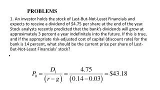
33. Problems • Ethanol solution of a dye (h=1.197 mPa·s) is used to feed a fluidic lab-on-chip laser. Dimension of the channel are L=122mm, width w=300um, height h=10 um. Calculate pressure required to achieve flow rate of Q=10ul/h. • 8.7 A soft drink with properties of 10 ºC water is sucked through a 4mm diameter 0.25m long straw at a rate of 4 cm3/s. Is the flow at outlet laminar? Is it fully developed? • Calculate total resistance of a microfluidic circuit shown. Assume that the pressure on all channels is the same and equal Dp.