Download
1 / 56
570 likes | 688 Vues
This paper presents an overview of the latest advancements in 3D sensor technology, focusing on improvements in speed related to current amplifiers and electrode designs. Significant factors affecting signal generation and amplification are discussed, including Ramo’s theorem and various electrode configurations such as trench and hex-cell sensors. Experimental results and analyses highlight the effectiveness of these innovations in reducing pulse collection times and enhancing signal clarity. The study aims to pave the way for future developments in high-speed 3D detection systems.

E N D
Speed: 3D sensors, current amplifiers Cinzia Da Via Manchester University Giovanni Anelli, Matthieu Despeisse1, Pierre Jarron CERN Christopher Kenney,Jasmine Hasi, SLAC Angela Kok SINTEF Sherwood Parker University of Hawaii Initial work and calculations with Julie Segal Wall electrode data with Edith Walckiers, Philips Semiconductors AG 1. now at Ecole Polytechnique Fédérale de Lausanne (EPFL), Institute of Microengineering (IMT), Photovoltaics and thin film electronics laboratory, Neuchatel, Switzerland.
1. introduction 2. history 3. factors affecting speed 4. generating the signal – Ramo’s theorem 5. amplifying the signal – charge and current amplifiers 6. trench electrode sensors 7. hex-cell sensors 8. experimental results 9. analysis – constant fraction discrimination 10. analysis – fitting with almost-noise-free pulses 11. next
Potential 3D features from preliminary calculations by Julie Segal: p 50 µm 8 µm n 50 µm 1 ns 3 ns 3. Fast pulses. Current to the p electrode and the other 3 n electrodes. (The track is parallel to the electrodes through a cell center and a null point. V – bias = 10V. Cell centers are in center of any quadrant. Null points are located between pairs of n electrodes.)
Speed: planar 3D 4. 4. 4. 1. 3D lateral cell size can be smaller than wafer thickness, so 2. in 3D, field lines end on electrodes of larger area, so 3. most of the signal is induced when the charge is close to the electrode, where the electrode solid angle is large, so planar signals are spread out in time as the charge arrives, and 4. Landau fluctuations along track arrive sequentially and may cause secondary peaks 5. if readout has inputs from both n+ and p+ electrodes, • shorter collection distance • 2. higher average fields for any given maximum field (price: larger electrode capacitance) • 3. 3D signals are concentrated in time as the track arrives • 4. Landau fluctuations (delta ray ionization) arrive nearly simultaneously • 5. drift time corrections can be made
1. introduction 2. history 3. factors affecting speed 4. generating the signal – Ramo’s theorem 5. amplifying the signal – charge and current amplifiers 6. trench electrode sensors 7. hex-cell sensors 8. experimental results 9. analysis – constant fraction discrimination 10. analysis – fitting with almost-noise-free pulses 11. next
A Very Brief History of Ever Shorter Times • The first silicon radiation sensors were rather slow with large, high capacitance elements. The resultant noise was reduced by integration. • For example, in the pioneering UA2 experiment at CERN, “the width of the shaped signal is 2 µs at half amplitude and 4 µs at the base.” (Faster discrete-component amplifiers were available, but not widely used.) • The development of microstrip sensors greatly reduced the capacitance between the top and bottom electrodes, adding a smaller, but significant one between adjacent strips. • The 128-channel, Microplex VLSI readout chip, had amplifiers with 20 –25 ns rise times, set by the need to roll off amplification well before • ω t ≤π (t = time, input to inverted output then fed back to input) • (Otherwise we would have produced a chip with 128 oscillators and no amplifiers.) • The planned use of microstrip detector arrays at colliders with short inter-collision times required a further increase in speed. • Silicon sensors with 3D electrodes penetrating through the silicon bulk allow charge from long tracks to be collected in a rapid, high-current burst. • Advanced VLSI technology provides ever higher speed current amplifiers. Up to the sensor speed, such signals grow more rapidly with increasing frequency, than white noise.
The first ever custom VLSI silicon microstrip readout chips. Made at Stanford in 1984). (left, 7.5 cm), then by AMI – (right, 10 cm).
planar sensor pulse shape (an early, successful, attempt to increase speed in the era of 1 μs shaping times) 30 ns 30 ns
1. introduction 2. history 3. factors affecting speed 4. generating the signal – Ramo’s theorem 5. amplifying the signal – charge and current amplifiers 6. trench electrode sensors 7. hex-cell sensors 8. experimental results 9. analysis – constant fraction discrimination 10. analysis – fitting with almost-noise-free pulses 11. next
Some elements affecting time measurements • variations in track direction – 1 and 2 can affect the shape and timing of the detected pulse. • variations in track location • variations in total ionization signal– can affect the trigger delay. • variations in ionization location along the track –Delta rays – high energy, but still generally non-relativistic, ionization (“knock-on”) electrons. Give an ever-larger signal when the Ramo weighting function increases as they approach a planar detector electrode, with their current signal dropping to zero as they are collected. This produces a pulse with a leading edge that has changes of slope which vary from event to event, limiting the accuracy of getting a specific time from a specific signal amplitude for the track. • magnetic field effects affecting charge collection –E× B forces shift the collection paths but for 3D-barrel only parallel to the track. • measurement errors due to noise – This currently is the major error source. • incomplete use of, or gathering of, available information – This is a challenge mainly for the data acquisition electronics which, for high speed, will often have to face power and heat removal limitations. • In addition, long collection paths for thick planar sensors increase the time needed for readout and decrease the rate capabilities of the system.
1. introduction 2. history 3. factors affecting speed 4. generating the signal – Ramo’s theorem 5. amplifying the signal – charge and current amplifiers 6. trench electrode sensors 7. hex-cell sensors 8. experimental results 9. analysis – constant fraction discrimination 10. analysis – fitting with almost-noise-free pulses 11. next
Calculating the signals • Calculate E fields using a finite element calculation. (Not covered here.) • Calculate track charge deposition using Landau fluctuating value for (dE/dx) divided by 3.62 eV per hole-electron pair. • Paths of energetic delta raysmay be generated usingCasino,a program from scanning electron microscopy. (GEANT4 may be used for some of 2 and 3.) • Calculate velocities and diffusion using C. Jacoboni, et al. “A review of some charge transport properties of silicon” Solid-State Electronics, 20 (1977) 7749. • Charge motion will induce signals on all electrodes, each of which will affect all the other electrodes. Handle this potential mess with: • Next: charge motion, delta rays, Ramo’s theorem.
≈ MeV; 1/Tmax ≈ 0 DELTA RAYS - 1 Integrating over T, the kinetic energy of the delta ray gives the number of delta rays in the 170 μm thickness of the hex sensor with T between T1 and T2 (Tmax is ≈ MeV; 1/Tmax ≈ 0) So 3 KeV δ rays are common, 30 KeV uncommon, 300 KeV rare. Calculate production angles and then look at some of them.
DELTA RAYS - 2 • With electron velocities of about 5 x 106 cm / sec, a delta ray of length 0.5 μm • if oriented ahead of the track • could reach an n electrode up to 10 ps ahead of the main track. • This will happen above 10 KeV in ≈ 5-10% of events • These energies will be compared with the mean loss • dE/dxmin, silicon = 1664 KeV / gm / cm2 giving • ΔTmean = 2.329 x 0.017 x 1664 = 65.9 KeV.
0.1µm 200 3-keV delta rays
1 µm 200 10-keV delta rays
15 µm 200 60-keV delta rays
Calculations based on material in: A REVIEW OF SOME CHARGE TRANSPORT PROPERTIES OF SILICON Solid-State Electronics 20 (1977) 77 – 89 C. Jacoboni, C. Canali, G. Ottaviani and A. Alberigi Quaranta
1. introduction 2. history 3. factors affecting speed 4. generating the signal – Ramo’s theorem 5. amplifying the signal – charge and current amplifiers 6. trench electrode sensors 7. hex-cell sensors 8. experimental results 9. analysis – constant fraction discrimination 10. analysis – fitting with almost-noise-free pulses 11. next
0.13 µm chips now fabricated and used here rise, fall times ≈ 1.5 ns rise times ≈ 3.5 ns fall times ≈ 3.5 ns
1. introduction 2. history 3. factors affecting speed 4. generating the signal – Ramo’s theorem 5. amplifying the signal – charge and current amplifiers 6. trench electrode sensors 7. hex-cell sensors 8. experimental results 9. analysis – constant fraction discrimination 10. analysis – fitting with almost-noise-free pulses 11. next
signal electrodes with contact pads to readout next section offset so signal electrodes do not line up 200 – 300 µm active edge beam in Schematic diagram of part of one section of two of the planes in an active-edge 3D trench-electrode detector. Other offsets (⅓, ⅔, 0, ⅓, ⅔ ..etc.) may also be used.
A trench-electrode sensor will have: • high average field / peak field, • a uniform Ramo weighting field, • an initial pulse time that is independent of the track position and, • for two facing 100 μm gaps with a common electrode and a 250 μm thickness (in the track direction)a capacitance of 0.527 pF per mm of height. • For moderate to high bias voltage levels ( ~ 50 V ) and low dopant levels ( ~ 5 x10¹¹ / cm3 ) we can neglect V depletion≈ 2 V, and assume a constant charge-carrier drift velocity. After irradiation, drift velocities will not be uniform, but will be faster as we raise the bias voltage.
nelectrode electrons Induced Current 100 μm holes p electrode time Schematic, idealized diagram of induced currents from tracks in a parallel-plate trench-electrode sensor. Tracks ( ● ) are perpendicular, at the mid and quarter points. Velocity (electrons) ≡ 3.0 × Velocity (holes).
SLAC Mask FE-I4 Sensor: 8 FE-I3 Sensors: 9 FE-I4 geometry test sensors: 55 Trench Sensors: 12: 50 um n-2-p pitch, 1 mm long, 64 channels 5: 50 um n-2-p pitch, 5 mm long, 64 channels 23: 100 n-2-p pitch, 3 mm long, 16 channels Talk title 28
Fast Timing Example Effort was made to pinch-off and isolate both types of trenches by deleting the surfaces of p-spray. So both electron and hole signals can be readout separately.
1. introduction 2. history 3. factors affecting speed 4. generating the signal – Ramo’s theorem 5. amplifying the signal – charge and current amplifiers 6. trench electrode sensors 7. hex-cell sensors 8. experimental results 9. analysis – constant fraction discrimination 10. analysis – fitting with almost-noise-free pulses 11. next
But for now we used a 50 μm-side hex sensor (following slides) 1. with 20 V bias, at room temperature - 40V should be ok, 2. with each column of hexagons tied to a 0.13 μm current-amplifier channel (so large capacitance), 3. exposed to an uncollimated 90Sr beta source, 4. output to an oscilloscope triggered by the signal itself.
1. introduction 2. history 3. factors affecting speed 4. generating the signal – Ramo’s theorem 5. amplifying the signal – charge and current amplifiers 6. trench electrode sensors 7. hex-cell sensors 8. experimental results 9. analysis – constant fraction discrimination 10. analysis – fitting with almost-noise-free pulses 11. next
a track in two and an induced pulse in the other (green) neighbor
First, one problem with betas: an example of a possible angled track distorting the pulse shape. (We will need real test beam data)
Uncollimated 90Sr betas, 20 C, hex sensor (20V bias) to 0.13 μm current amplifier, self-triggers, event 1 of 99 30 ns
Uncollimated 90Sr betas, 20 C, hex sensor (20V bias) to 0.13 μm current amplifier, self-triggers, event 99 of 99 30 ns
The single-column event with the largest expected timing error in the central scatter plot.
30 ns Pulse shape from the sum of the 6 largest pulses. τ-rise = 1.6 ns, fwhm = 2.90 ns. Note the trailing edge hole current, and amplifier ringing.
With a pulse from a pulse generator, with the 10% and 90% time points only 0.8 ns apart, we see an amplifier rise time of 1.5 ns. Sensor signals have rise times of 1.6 ns. So the amplifier is currently the limiting element.
1. introduction 2. history 3. factors affecting speed 4. generating the signal – Ramo’s theorem 5. amplifying the signal – charge and current amplifiers 6. trench electrode sensors 7. hex-cell sensors 8. experimental results 9. analysis – constant fraction discrimination 10. analysis – fitting with almost-noise-free pulses 11. next
ΔT σ-noise • Estimate the time resolution at room temperature with • the hex sensor, and • a preliminary version of a 0.13 µm integrated circuit readout • using data from un-collimated 90-Sr βs (but only with tracks in the central channel). • (A wall-electrode with parallel plates would give shorter times, but the hex sensor already has almost the same output rise time as a 0.8 ns input rise time pulse generator, so the output shape is primarily determined by the amplifier, not the sensor). • To simulate a constant fraction discriminator set at 50% (where slope is steepest): • Fit leading baseline, and measure noise, • Fit top and find halfway point, • ΔT = σ-noise / slope • With wall-electrode sensor and a parallel beam, • can do better fitting entire pulse.
Noise distribution from pre-pulse region with a Gaussian fit.
Noise distribution from pre-pulse with a Gaussian fit – log scale to show tails sigma = 0.33166 +/- 0.0033 mV direct standard deviation from the18,090 voltage values = 0.3218 mV
Scatter plot of expected noise-induced timing errors, dt, vs. pulse amplitude, for 67 pulses and the projections of dt and amplitude distributions. σ (noise) = 0.33 mV. dt σ noise