Modeling Seasonal Trends and Interannual Differences in Cod Biomass Cohorts Growth
This study analyzes the seasonal trends and interannual differences in the biomass of cod cohorts using Growth Models (Gi and GAMs). The findings highlight strong seasonal influences on growth and mortality rates, showing that variability in biomass is more significantly impacted by fixed solar cycles than by temperature. The research underscores the necessity of low mortality and rapid growth for producing strong year-classes, while also identifying the relevant environmental factors affecting cod populations over different years.

Modeling Seasonal Trends and Interannual Differences in Cod Biomass Cohorts Growth
E N D
Presentation Transcript
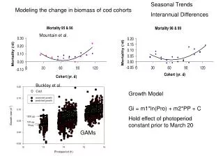
Seasonal Trends Interannual Differences Modeling the change in biomass of cod cohorts Mountain et al. Buckley et al. Growth Model Gi = m1*ln(Pro) + m2*PP + C Hold effect of photoperiod constant prior to March 20 GAMs
Modeling the change in biomass of cod cohorts Mi = m1*cohort + m2*(cohort)3 + C Low (98+99) or High (95+96) M G Gi = m1*ln(Pro) + m2*PP + C Poor (95) or Fast (99) M/G High Mortality with 1995 Growth Biomass March February April April May
Conclusions Strong seasonal trends in growth and mortality rates Large interannual differences Position in fixed solar cycle explains more variability in M and G than temperature Low mortality and rapid growth are necessary but not sufficient for production of a strong year-class