ATLAS Experiment Silicon Detector Alignment
1. ATLAS Experiment Silicon Detector Alignment. IPRD06. Müge KARAG Ö Z ÜNEL the University of Oxford for the ATLAS Silicon Alignment Community. IPRD06, Siena, Italy October 1-5, 2006. MKU. 8 SCT modules. 6 PIXEL modules. y. x. z. 2. The Prelude. Surface Cosmic.

ATLAS Experiment Silicon Detector Alignment
E N D
Presentation Transcript
1 ATLAS Experiment Silicon Detector Alignment IPRD06 Müge KARAGÖZ ÜNEL the University of Oxford for the ATLAS Silicon Alignment Community IPRD06, Siena, Italy October 1-5, 2006 MKU
8 SCT modules 6 PIXEL modules y x z 2 The Prelude Surface Cosmic Combined Test Beam IPRD06 All results are preliminary. There will be a bias will towards cosmic results and global chi2 algorithm. For information on the SCT+Pixel hardware, installation and performance, see Sergio Sevilla, Harald Fox and Andreas Korn’s talks. ATLAS Pit MKU
TRT Pixels (3 layers+3 disks) SCT endcaps: 9 disks SCT barrels: 4 layers 3 The Challenge: Atlas Silicon is BIG! IPRD06 3 translations & 3 rotations of each module MKU In total we have to deal with 34,992 DoF’s!
4 The Strategy: Various Approaches • Prerequisite: need to cope with the demands of ATLAS physics requirements • intrinsic alignment of Si (offline, online, survey) • Si+TRT (help sagitta, etc..) • Methods: all rely on track residual information • Global 2: • minimization of 2 fit to track and alignment parameters • 6 DoF, correlations managed, small number of iterations • Inherent challenge of large matrix handling and solving • Local 2 : • similar to global 2, but inversion of 6x6 matrix per module • 6 DoF, no inter-module or MCS correlations, i.e. diagonal covariance matrix • large number of iterations • Robust Alignment: • use weighted residuals, z and rphi overlap residuals of neighboring modules • 2-3 DoF, many iterations, no minimization • Valencia Alignment (used mainly for CTB): • Numerical 2 minimization • 6 DoF, many iterations IPRD06 MKU
5 Algorithms’ Functionalities • All algorithms are implemented within ATLAS framework and able to use the common tracking tool and database • Functionalities exist to add constraints from physics& external data (vertex, mass requirements, online alignment and survey data) for the global and/or local chi2 minimization algorithms IPRD06 Tracks in StoreGate Digits Reconstruction Alignment Algorithm Iteration until convergence, N_iter different for all algorithms Alignment Constants Final Alignment Constants MKU
track Intrinsic measurement error + MCS hit residual Key relation! 6 Global 2 approach The method consists of minimizing the giant 2resulting from a simultaneous fit of all particle trajectories and alignment parameters: Let us consequently use the linear expansion (we assume all second order derivatives are negligible). The track fit is solved by: IPRD06 while the alignment parameters are given by: MKU Equivalent to Millepede approach from V. Blobel
8 (-1) SCT Modules (1 dead) 6 PIXEL modules y x z 7 Combined Test Beam (2004) • First real data from ID subsystems! • Abundant statistics of e+/e- and pions (2-180 GeV) (O(105) tracks/module/E), • Magnetic field on/off runs. • Limited setup and layout, creating systematic effects in modes • A good start to test algorithms for more realistic upcoming data! IPRD06 • Algorithms use different approaches in extracting alignment constants: various DoF, (un/)biased residuals, etc.. • All algorithms improve residuals and quality of the track parameters significantly. Consistent results within slight differences (likely to be attributed to global transformations) • Ongoing efforts to combine/compare results of the algorithms. MKU
8 CTB – Performances - I • Robust: • converge after about 15 iterations • only detector plane alignment (X,Y) • after alignment, pixel residuals 0(10m) • Local chi2: • converge after about 15 iterations • after alignment, SCT residuals are O(25m) and pixels are 0(10m) IPRD06 SCT 3D unbiased residuals – run 2102365 Iteration 1 and 15 PIXEL Before After MKU
=19.1 μm 9 CTB – Performances - II • Global chi2: on 3DoF (detector plane, TX,TY,RZ), quick convergence • results with anchorage or no anchorage • overall pixel residual mean is 10.7 mum and SCT is 19.1 mum SCT after SCT before IPRD06 • Valencia: • align pixel first, then SCT, then all • first pixel as anchor, • many iterations MKU
Use CTB Straightlinefitter Loss of efficiency for small d0 and large phi0 10 ID Cosmic Run (2006) Scint 1 • Data-taking at surface (SR1) in spring 2006: ~400k events recorded! • 22% of SCT Barrel: 467 instrumented modules • 13% of TRT Barrel • 3 (or 2) Scintillators to trigger 144cmx40cmx2.5cm • Trigger Time resolution ~ 0.5ns: ~ 3-400MeV cutoff for alignment studies • No B-field! No momentum! MSC important ~<10 GeV, need to deal with large residuals IPRD06 Scint 2 floor acts as absorber for p< 170 MeV Scint 3 MKU
11 SR1 Cosmics: global 2 - real data 2808 DoF’s, ~250k tracks Before alignment After alignment Corrections due to modes >1500 IPRD06 first iteration Corrections x100 Alignment corrections for rigid barrels =46 μm =31.9 μm TX TY TZ RX RY RZ [mm] [mm] [mm] [mrad] [mrad] [mrad] Barrel3 -0.0044 -0.0162 -0.0169 0.0685 -0.0185 0.0503 Barrel4 0.0061 0.0329 -0.0462 -0.0678 0.0258 0.0527 Barrel5 0.0109 -0.0005 0.0865 0.0318 -0.0134 -0.0947 Barrel6 -0.0126 -0.0162 -0.0234 -0.0200 0.0073 -0.0083 Indication of very good assembly precision! Better than misaligned simulation! MKU
12 SR1 Cosmics: global 2 - real data systematic effects visible when only 6 modes removed First iteration Third iteration Correction x100 IPRD06 before after MKU
13 SR1 Cosmics: global 2 - simulated data Perfectly aligned detector, but still minor bugs in detector descriptions =31.2 μm IPRD06 Traces of systematics??? Beware: Alignment is ultimately sensitive to own bugs and approximations but also to slightest upstream imperfections. Sometimes hard to tell apart! MKU
14 SR1 Cosmics: local 2 Alignment of SCT barrel cosmic test setup with 36k tracks. Flow of alignment parameter ax for all modules of barrel layer 2 through the iterations IPRD06 BEFORE AFTER MKU =113.8 -> 80.0 80.9 μm =99.5 -> 75.5 64.8 μm =96.1 -> 64.7 71.1 μm =111.2 -> 85.7 70.9 μm rnd misal:
15 SR1 Cosmics: Robust alignment • The method works on the cosmic setup, ongoing studies with refitted tracks. 10k tracks After 8 iterations: RMS residual 61µm → 47µm IPRD06 After 8 iterations: RMS overlap residual 81µm → 69µm MKU
16 Nominal Detector Simulation: Global 2 x100 • 1M muon sample (~8M tracks in full fiducial) generated for ATLAS Computing Challenge. The largest sample looked currently! • Align 2172 Barrel SCT+PIX modules in |eta|<1 (“Double Cone”), 13032 DoF • Solution using ScaLAPACK on an AMD Opteron ||-cluster (< ½ hour). • Systematic effects in Pixels which was not visible to earlier studies: statistics washed out or sth new? • Disappear after cut on low freq. modes (i.e., global effect) • Special misalignments can also be introduced in three levels: • module level, layers&disks, Silicon ID subsystems • Data analysis of this is ongoing.. IPRD06 x100 MKU
17 Nominal Detector Simulation: Global 2 PIXEL IPRD06 x100 PIXEL Pulls in diagonal base Pulls of alignment corrections Typical errors < 10μm MKU
Time FSI months Tracks days hours minutes seconds Barrel SCT Spatial frequency eigenmode 80+(3x[80+16])+(2x72)=512 End-cap SCT 165x2=330 18 Including online alignment: FSI • On-detector geodetic grid of 842 simultaneouslength measurements (precision <1m ) between nodes on SCT support structure. • Grid shape changes determined to <10m in 3D. • Time + spatial frequency sensitivity of FSI complements track based alignment: • Track alignment average over ~24hrs+. high spatial frequency eigenmodes, “long” timescales. • FSI timescale (~10mins) low spatial frequency distortion eigenmodes (e.g. sagitta). • Need both! • First principles studied, implementation work is to be performed! IPRD06 MKU
19 Summary & Conclusions • Various algorithms are adapted to optimally align ATLAS ID. • Algorithms have proved proof of principles. • Codes have been continuously implemented and heavily tested. • We have been looking at real data already! • At SR1 data taking, SCT barrel was found to be built very well! • CTB efforts are almost finalized. • Cosmic alignment progressing rapidly. • We are on our way to understand and tackle many systematic issues, both in real data and simulation, upstream and downstream of alignment algorithms… • Pixels and endcaps are getting ready for cosmic data. • FSI is getting ready for monitoring during pixel insertion in pit. • Stay tuned! IPRD06 MKU
20 We are… • The Silicon alignment team • Pawel Bruckman, Stephen Gibson, Tobias Golling, Carlos Escobar, Richard Hawkings, Roland Heartel, Florian Heinemann, Adlene Hicheur (ex), MKU, Stefan Kluth, Salva Marti Garcia, Bjarte Mohn, Ola K. Oye, Sergio Gonzalez Sevilla, Jochen Schiek, (am surely missing a few, please help me finalize this list!) • And • The hardware and DAQ teams of all setups • Reconstruction groups • CERN crew for installation and survey data • More information: • https://uimon.cern.ch/twiki/bin/view/Atlas/InDetAlignment IPRD06 MKU
21 BACKUP Si modules CTB+SR1 Details Global chi2 details Full barrel solution Robust align. details FSI Details Survey Data IPRD06 MKU
Si Sensors Hybrid with ASICs ASICs ~70mm ~140mm Si Sensor TPG+BeO Baseboard 22 Building blocks of SCT IPRD06 • PIXel detectors provide real 2-D readout (size 50400 m resulting in 14115 m resolution). • SCT modules are double-sided strip detectors with 1-D RO/side (768 instrumented strips). • Sensitive strips have pitch of 80 m giving 23 m resolution. • Stereo-angle of 40 mrad gives 580 m resolution in the other direction. • Entire Si tracker is equipped with binary RO chips. • SCT end-cap modules are different in shape: wedged structure MKU
23 Weak distortional modes (ex.) IPRD06 “clocking” R (VTX constraint) radial distortions (various) “telescope” z~R • dependent sagitta • XabRcR2 • We need extra handles in order to tackle these. Candidates: • Requirement of a common vertex for a group of tracks (VTX constraint), • Constraints on track parameters or vertex position (external tracking (TRT, Muons?), calorimetery, resonant mass, etc.) • Cosmic events, • External constraints on alignment parameters (hardware systems, mechanical constraints, etc). • dependent sagitta “Global twist” • Rcot() MKU
24 Global chi2: more on modes Example “lowest modes” in PIX+SCT Global Freedom have been ignored (only one Z slice shown) IPRD06 • The above “weak modes” contribute to the lowest part of the eigen-spectrum. Consequently they dominate the overall error on the alignment parameters. • More importantly, these deformations lead directly to biases on physics (systematic effects). MKU
25 Robust alignment: constants Sum over neighbours, take correlations into account IPRD06 Sum over all modules in a ring Correct for change in radius For a perfect detector: MKU
26 Solving the full system • Global 2 formalism requires solving large number of LE and handling large sized-matrices. • Limiting factors: • Size: * Solving full ID needs 9.8GB. By default, Atlas software infrastructure allows only 2GB of memory/job on 32-bit machines. • Precision: Conventional 32-bit libraries are not fully adequate for full size solution accuracy. Alignment matrices can have large condition numbers (compete with machine precision.) • Execution time: Single-CPU machines with unoptimized libraries can take number of hours to solve large-size problems. • Currently using 64-bit //-computing: a huge improvement. • Solving full pixel (2112 modules, 12.5k DoF) on 16 nodes takes 10mins compared with 7hrs on Intel P4 • And solving full system was not even possible until last year! • Work ongoing on other methods for further improvement: • Various investigations on iterative methods • Plan to implement one such method (MA27) in athena • plan to port code on 64-bit to do processing+solving all at once. IPRD06 MKU
27 Nominal Detector Simulation: Global chi2 Full barrel i.e. 21408 DoF’s. IPRD06 pdsyevd of ScaLAPACK on a 64bit ||-cluster AMD Opteron. Using 16 CPU grid N=21k system diagonalised within ~1h! =0.94 Pulls in diagonal base Pulls of alignment corrections Pulls of all corrections of ~unit width and centred at zero MKU
28 CTB Setup IPRD06 MKU
29 SR1 Cosmics: Readout • SCT inserted into the TRT on17/02/2006 • Physics mode data coming in end of april until june 2006. • SCT read 3 time bins (75nsec) and accept any hit in these three time bins • TRT: read every 3.125nsec and 24 time bins (75 nsec). IPRD06 MKU
30 SR1 Cosmics : Hitmap From simulation IPRD06 MKU
31 Online alignment: FSI IPRD06 MKU
FSI grid nodes attached to inner surface of SCT carbon-fibre cylinder Distance measurements between grid nodes precise to <1 micron 32 On-detector FSI System IPRD06 MKU
FSI interferometer data Length extraction FSI Grid Lengths Reconstruction Interpolation Grid Node DoF Module corrections 33 FSI Analysis Chain ~400MB per scan (one scan upto every 10 minutes) only every Nth scan archived Most CPU intensive meta data ~300 kB Lengths + errors: 12.6kB IPRD06 Model configuration data (TBD) +2MB laser configuration data -> either configuration db or some local file Nodes + errors 9.6kB Model configuration data (TBD) MKU (192 kB per scan) ~<9.6kB eigenmode amplitudes
34 FSI + Track alignment • How to include time dependency? • FSI provides low spatial frequency module corrections at time ti , t0<ti<t1 • Track recorded at time ti is reconstructed using FSI module correction at time ti . • Global (or robust) Chi sq uses FSI corrected tracks to construct chi sq and minimises to solve for high spatial frequency modes, averaged over t0<ti<t1, low frequency modes frozen. • Subsequent reconstruction of track at time tj uses average alignment from global (or robust) chi sq + time dependent FSI module correction, tj, t0<tj<t1 IPRD06 Global Chi2 can add extra terms to the weight matrix and the big vector of the final system of equations to incorpoarate external FSI constraint MKU
35 SR1 SCT+TRT photogrammetry • SCT Barrel photogrammetry survey was completed early this year. • SCT-TRT relative position survey also performed. IPRD06 MKU
36 Photogrammetry: Deformations • Measurements performed before and after insertion into TRT. Detailed measurements exist only before the insertion O(20μm) in XY. • After insertion only coordinate system transfer was measured. • The individual cylinder interlink data showed deformations consistent with tilted ellipses. • Face A and face C appear to be rotated in opposite directions, hinting at twists of the complete barrel. Deformations are order of 100 μm. B3 B4 IPRD06 B5 B6 Circles (colored) are fits, black curves are guidelines for ellipses using the scaled up differences of data points (col) to the circles MKU