Download
1 / 53
530 likes | 563 Vues
This Master's Thesis Defense explores using Large-Eddy Simulations to study microphysical behavior in midlevel, mixed-phase clouds. Analyzing cloud cases, budget analysis, developing analytic equations, and verification are discussed. The study focuses on the importance of cloud phase in climate models, with implications for radiation budget and aircraft safety. The research aims to predict cloud phase behavior accurately.

E N D
Using Large-Eddy Simulations to analyze microphysical behavior in midlevel, mixed phase clouds Master’s Thesis Defense Adam J. Smith The University of Wisconsin-Milwaukee November 28, 2007
Outline • Introduction • Numerical model description • Cloud cases • Budget analysis • Development of analytic equations • Verification of analytic equations • Conclusions / Future work
What are midlevel “alto” clouds? • Thin clouds (less than 1 km thick) • Generally overcast • Often mixed phase • Occur in any climate region (Sassen and Khvorostyanov, 2007) • Cover up to 22% of the planet’s surface (Warren et al., 1988)
The importance of cloud phase • Climate models and general circulation models (GCMs) have difficulty predicting cloud phase (liquid, ice, or both) • Significant effect on radiation budget • Variations in glaciation temperature lead to an 8 W m-2 difference in shortwave cloud radiative forcing (Fowler et al., 1996) • Ackerman et al. (2004): “One key area that impacts cloud feedbacks to climate is the phase [of clouds]”.
What about other effects? • Icing threat to small aircraft • During Operation ENDURING FREEDOM, three Air Force Predator aircraft crashed in Afghanistan due to icing (Haulman, 2003) • Unmanned aerial vehicles (UAVs) often operate at altitudes where mixed-phase alto clouds exist • In a study of aircraft icing environments, 48% of observed environments in temperature range of 0 to -30°C were mixed-phase (Cober and Isaac, 2002)
The “forgotten clouds” • Vonder Haar et al. (1997) call mid-level alto clouds “the forgotten clouds” because they are under-studied. • Zhang et al. (2005) find that GCMs greatly underpredict thin alto clouds while overpredicting thicker clouds like nimbostratus • Nimbostratus are primarily comprised of liquid, which have different reflective properties than ice or mixed-phase clouds • Methods must be devised to predict cloud phase and overcome prediction issues
“Can we predict phase in asimple but informative way?” • Simulate three mixed-phase alto clouds observed by aircraft • Simulations are high-resolution and three-dimensional, with full microphysics • Budget equations determine the important effects • Analyze changes in liquid and snow mixing ratio • What processes cause these changes? • Develop analytic equations to predict phase behavior • Equations only require a few inputs • Inputs can be estimated instead of directly measured
Outline • Introduction / Rationale • Numerical model description • Cloud cases • Budget analysis • Development of analytic equations • Verification of analytic equations • Conclusions / Future work
Numerical model • We select the Coupled Ocean/Atmospheric Mesoscale Prediction System (COAMPS®) Large Eddy Simulation (COAMPS-LES) model (Golaz et al., 2005). • Model was previously used to perform detailed three-dimensional studies (e.g. Larson et al., 2006; Falk and Larson, 2007).
General model settings • Simulation length: 4 hours • Time step: 1 s • Vertical grid spacing: 25 m • Horizontal grid spacing: 75 m • Horizontal domain size: 4125 m x 4125 m • Vertical domain size: 4400 m – 4500 m (varies) • 1-hour spinup period for turbulence • Microphysics activated at t = 61 min • Second 30 min spinup period for microphysics
Microphysics scheme • Based on Rutledge & Hobbs (1983), subsequently referred to as RH83 • Single-moment bulk microphysics equations • Predicts mixing ratios, but uses diagnostic formulas to determine ice mass, number concentration, diameter, fallspeed, etc. • More advanced schemes actively predict these parameters, but at a much greater computational cost • Five hydrometeor species: cloud water (rc), rain (rr), cloud ice (ri), snow (rS), graupel (rg) • Microphysical processes: collection, depositional growth, sublimation • Aggregation is not used in this microphysical scheme • Graupel and rain deactivated (not detected in observations)
Ice particle number concentration • Ice particle number concentration: greatest of values calculated using Fletcher (1962) and Cooper (1986) formulas. • Concentration is a diagnostic function of temperature; not directly affected by microphysics calculations • This method provides no sinks of ice nuclei • Does not produce major errors in simulation
Outline • Introduction / Rationale • Numerical model description • Cloud cases • Budget analysis • Development of analytic equations • Verification of analytic equations • Conclusions / Future work
Cloud cases • Three mixed-phase cloud cases: • 11 November 1999 (denoted Nov.11 case) • 14 October 2001 (denoted Oct.14 case) • 02 November 2001 (denoted Nov.02 case) • All cases were observed by aircraft during the Complex Layered Cloud Experiments (CLEX) • All are “altostratocumulus” (Larson et al., 2006) • Overcast (like “stratocumulus”) • Isolated from boundary layer (hence “alto”) • “Altocumulus” consist of “distinct elements”, while our cases are stratiform • Peak liquid at cloud top, peak snow near cloud base
Nov. 11 case (11 November 1999) • Sampled during CLEX-5 over central Montana • Studied previously in Larson et al. (2006) • Sampling occurred from 1224 – 1336 local time • Cloud region dissipated during sampling (Fleishauer et al., 2002) • Liquid layer: 500 m thick • Large scale ascent: -3 cm s-1 • Constant solar zenith angle (observed near midday) • No induced vertical wind profile in simulation (lack of vertical wind shear)
Oct. 14 case (14 October 2001) • Observed during CLEX-9 over central Nebraska • Sampled from 0610 – 1000 and 1115 – 1300 local time (sunrise through midday) • Satellite observations show cloud region persists through sampling periods (not shown) • Liquid layer: 800 m thick • Ice layer: extends 2000 m below liquid • Above- and below- cloud data from supplemental sounding • Launched at NWS site on Lee Bird Field (LBF), North Platte, NE • 45 miles away from aircraft observation location • Varied solar zenith angle using Liou (2002) • Ascent of 1.4 cm s-1 (obtained from NCEP North American Regional Reanalysis)
Nov. 02 case (02 November 2001) • Also observed during CLEX-9 over central Nebraska • Sampled from 0620 – 1020 local time (sunrise through mid-morning) • Satellite images indicate cloud region dissipated by 1230 local time (not shown) • Warmer temperatures than Oct.14 case • Liquid layer: only 400 m thick • Ice layer: extends 1500 m below liquid • Again, supplemental sounding launched at LBF • Varied solar zenith angle • Ascent of 0.7 cm s-1
Verification methods 1. Comparisons of observed versus simulated profiles at end of spinup (t = 61 min) • Simulated profiles tuned to match observations 2. Comparisons of observed versus simulated snow mixing ratio at t = 90 min • Snow profiles NOT tuned to match observations • t = 90 min is selected to account for microphysical spinup 3. Examination of time series evolution for liquid and snow
Outline • Introduction / Rationale • Numerical model description • Cloud cases • Budget analysis • Development of analytic equations • Verification of analytic equations • Conclusions / Future work
Budget analysis • Which model processes are important? • We evaluate budget equations • Large scale and microphysical processes included • We focus primarily on microphysics • Small or negligible contributions neglected • Individual budget terms (including negligible terms) add up to equal total tendency • Cloud water and snow budgets are examined • We observe from t = 91 min to t = 150 min, to account for microphysical spinup
Budget equations where: Mix = change due to turbulent mixing Ascent = change due to large-scale ascent Rad = change due to radiative forcing Sediment = change due to the motion of falling snow (“sedimentation”) PSACW = change due to snow collecting cloud water PSDEP = change due to depositional growth of snow PDEPI = change due to depositional growth of cloud ice PCONV = conversion of cloud ice to snow
Major observations from budgets • Most important microphysical process: Depositional growth of snow • Other microphysical processes generate smaller effects • Balance between depositional growth of snow and sedimentation in Oct.14 and Nov.02 cases • Time tendency of snow is relatively small, except with strong descent in Nov.11 case
Outline • Introduction / Rationale • Numerical model description • Cloud cases • Budget analysis • Development of analytic equations • Verification of analytic equations • Conclusions / Future work
Analytic equations • Useful to predict snow mixing ratio and precipitation flux • Analytic equations allow for simple predictions without a lot of information • Formulas are derived from RH83
Simplified snow budget • Presumptions: • Sedimentation balances depositional growth exactly • Steady state processes (no time tendency) • Other microphysical terms are negligible
Analytic formulas • Unknown variables: • p (pressure) • ρ (air density) • T (temperature) • ztop (liquid cloud top altitude) • z (liquid cloud base altitude) • Si (fraction of saturation with respect to ice) • esi (saturation vapor pressure) • By using a reasonable estimate for each unknown variable, we can explicitly solve these equations.
Outline • Introduction / Rationale • Numerical model description • Cloud cases • Budget analysis • Development of analytic equations • Verification of analytic equations • Conclusions / Future work
Methods for verifying analytic formula • Completed a series of sensitivity simulations • No collection processes used in study • Adjusted variables: • Large scale ascent • Variable a’’ (affects snow fall velocity) • Variable N0S (affects snow particle number concentration) • Total number of sensitivity simulations: 17 different settings x 3 cloud cases = 51 total
Formula verification • For each simulation, observation time is based on when peak snow mixing ratio occurs • Diagnosed value of snow mixing ratio and snow precipitation flux obtained directly from simulation results • Analytic results also calculated with inputs from simulation • Results plotted using scatter plot
Formula underpredicts mixing ratio Line indicates equality Formula overpredicts mixing ratio
Formula underpredicts mixing ratio Line indicates equality Formula overpredicts mixing ratio
Formula underpredicts mixing ratio Line indicates equality Formula overpredicts mixing ratio
Formula underpredicts mixing ratio Line indicates equality Formula overpredicts mixing ratio
Results from our verification • Formulas consistently underpredict snow mixing ratio and precipitation flux • Underprediction is likely due to neglected terms, especially time tendency • We still need to evaluate tendencies of the individual results • A multiplicative or additive factor could be useful
Outline • Introduction / Rationale • Numerical model description • Cloud cases • Budget analysis • Development of analytic equations • Verification of analytic equations • Conclusions / Future work
Conclusions • For this study, we simulate three mixed-phase alto clouds • Depositional growth is the strongest microphysical process affecting liquid and snow • Sedimentation of snow nearly balances depositional growth • Time tendency of snow mixing ratio is nearly zero in two simulations • A series of simple analytic equations was derived from budget observations. • Analytic equations require inputs that can easily be estimated • Equations consistently underestimate snow properties, but they still provide accurate and useful information.
Future work • Examine log-log plot results more closely • Why does the analytic formula produce different results when the simulation predicts almost exactly the same value? • Can we factor time tendency into our equations? • What about other neglected terms? • How do equations perform when analyzing different snow habits? • Test equations versus a more robust microphysics scheme.
Acknowledgements • Professor Vince Larson for advising my research • My research associates: Michael Falk, Dave Schanen, Brian Griffin, Brandon Nielsen, and Joshua Fasching for working with me on various computer and scientific issues • Dr. Jean-Christophe Golaz (NOAA / GFDL) for providing technical assistance with COAMPS-LES • Dr. Larry Carey (ESSC / Univ. of Alabama Huntsville), Dr. Jingguo Niu (Texas A&M Univ.), and Dr. J. Adam Kankiewicz for providing vital aircraft and rawinsonde data • My fellow graduate students, family, friends, and my fianceé Apryle • Viewers Like You • COAMPS® is a registered trademark of the Naval Research Laboratory