
SlideServe
Menu
Préférences
© SlideServe · v2026

Kalman Filter Homework 2

emile avatar
4 diapositives · 268 Views · Aug 01, 2014

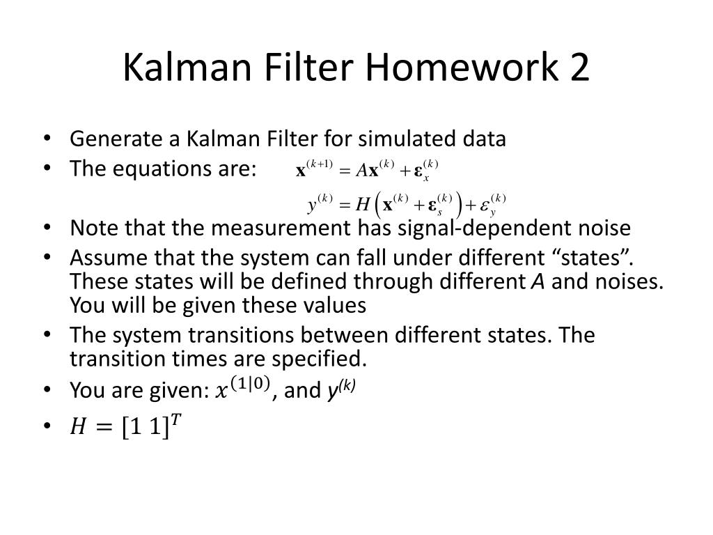
Kalman Filter Homework 2. Generate a Kalman Filter for simulated data The equations are: Note that the measurement has signal-dependent noise
Kalman Filter Homework 2 - slide 1
01 / 4Kalman Filter Homework 2
1 / 17

Télécharger la présentation

Kalman Filter Homework 2
Une image / un lien ci-dessous est fourni (tel quel) pour télécharger la présentation

Politique de téléchargement : le contenu du site vous est fourni TEL QUEL pour votre information et votre usage personnel ; il ne peut être vendu, concédé sous licence ni partagé sur d’autres sites sans l’accord de son auteur.Le contenu vous est fourni TEL QUEL, pour votre information et votre usage personnel uniquement. Téléchargez la présentation en cliquant sur ce lien. Lors du téléchargement, si vous ne parvenez pas à télécharger une présentation, l’éditeur a peut-être supprimé le fichier de son serveur.Pendant le téléchargement, si vous ne parvenez pas à obtenir une présentation, le fichier a peut-être été supprimé par l’éditeur.

F I N

Plus de contenu associé

Transcription de la présentation
  1. Kalman Filter Homework 2 • Generate a Kalman Filter for simulated data • The equations are: • Note that the measurement has signal-dependent noise • Assume that the system can fall under different “states”. These states will be defined through different A and noises. You will be given these values • The system transitions between different states. The transition times are specified. • You are given:, and y(k)

  2. States

  3. State 1 State 2 State 3 State 4

  4. Task: • For each state, defined on the next slide, calculate the steady state that the Kalman Gain will converge to. • Write and implement a Kalman Filter. Note that the measurement noise is signal-dependent. • At each state transition, change your A matrix and noises appropriately • Your estimates of x and P at the end of each state will carry over into the next state. • Compare your final Kalman Gain at the end of each state with your analytically calculated value • Also compare the Kalman Gain at each iteration to the “gain” of an LMS algorithm (plot and compare these two gains)