High-Performance, Power-Aware Computing

1. High-Performance, Power-Aware Computing Vincent W. Freeh Computer Science NCSU vin@csc.ncsu.edu

2. Acknowledgements • Students • Mark E. Femal – NCSU • Nandini Kappiah – NCSU • Feng Pan – NCSU • Robert Springer – Georgia • Faculty • Vincent W. Freeh – NCSU • David K. Lowenthal – Georgia • Sponsor • IBM UPP Award

3. The case for power management in HPC • Power/energy consumption a critical issue • Energy = Heat; Heat dissipation is costly • Limited power supply • Non-trivial amount of money • Consequence • Performance limited by available power • Fewer nodes can operate concurrently • Opportunity: bottlenecks • Bottleneck component limits performance of other components • Reduce power of some components, not overall performance • Today, CPU is: • Major power consumer (~100W), • Rarely bottleneck and • Scalable in power/performance (frequency & voltage) Power/performance “gears”

4. Is CPU scaling a win? • Two reasons: • Frequency and voltage scaling Performance reduction less than Power reduction • Application throughput Throughput reduction less than Performance reduction • Assumptions • CPU large power consumer • CPU driver • Diminishing throughput gains power (1) CPU power P = ½ CVf2 performance (freq) application throughput (2) performance (freq)

5. AMD Athlon-64 • x86 ISA • 64-bit technology • Hypertransport technology – fast memory bus • Performance • Slower clock frequency • Shorter pipeline (12 vs. 20) • SPEC2K results • 2GHz AMD-64 is comparable to 2.8GHz P4 • P4 better on average by 10% & 30% (INT & FP) • Frequency and voltage scaling • 2000 – 800 MHz • 1.5 – 1.1 Volts

6. LMBench results • LMBench • Benchmarking suite • Low-level, micro data • Test each “gear”

7. Operations

8. Operating system functions

9. Communication

10. Energy-time tradeoff in HPC • Measure application performance • Different than micro benchmarks • Different between applications • Look at NAS • Standard suite • Several HP application • Scientific • Regular

11. +66% +15% +25% +2% +150% +52% +45% +8% +11% -2% Single node – EP • CPU bound: • Big time penalty • No (little) energy savings

12. Single node – CG +1% -9% +10% -20% • Not CPU bound: • Little time penalty • Large energy savings

13. Operations per miss • Metric for memory pressure • Must be independent of time • Uses hardware performance counters • Micro-operations • x86 instructions become one or more micro-operations • Better measure of CPU activity • Operations per miss (subset of NAS) • Suggestion: Decrease gear as ops/miss decreases

14. Single node – LU +4% -8% +10% -10% Modest memory pressure: Gears offer E-T tradeoff

15. Ops per miss, LU

16. Results – LU Shift 0/1 +1%, -6% Gear 1 +5%, -8% Shift 1/2 +1%, -6% Gear 2 +10%, -10% Auto shift +3%, -8% Shift 0/2 +5%, -8%

17. Bottlenecks • Intra-node • Memory • Disk • Inter-node • Communication • Load (im)balance

18. S8 = 7.9 S2 = 2.0 S4 = 4.0 Perfect speedup: E constant as N increases E = 1.02 Multiple nodes – EP

19. S8 = 5.3 E8 = 1.16 Gear 2 Multiple nodes – LU S8 = 5.8 E8 = 1.28 S4 = 3.3 E4 = 1.15 S2 = 1.9 E2 = 1.03 Good speedup: E-T tradeoff as N increases

20. Multiple nodes – MG Poor speedup: Increased E as N increases S8 = 2.7 E8 = 2.29 S4 = 1.6 E4 = 1.99 S2 = 1.2 E2 = 1.41

21. Normalized – MG With communication bottleneck E-T tradeoff improves as N increases

22. Can increase N decrease T and decrease E Jacobi iteration

23. Future work • We are working on inter-node bottleneck

24. Safe overprovisioning

25. The problem • Peak power limit, P • Rack power • Room/utility • Heat dissipation • Static solution, number of servers is • N = P/Pmax • Where Pmax maximum power of individual node • Problem • Peak power > average power (Pmax > Paverage) • Does not use all power – N * (Pmax - Paverage) unused • Under performs – performance proportional to N • Power consumption is not predictable

26. Safe over provisioning in a cluster • Allocate and manage power among M > N nodes • Pick M > N • Eg, M = P/Paverage • MPmax > P • Plimit = P/M • Goal • Use more power, safely under limit • Reduce power (& peak CPU performance) of individual nodes • Increase overall application performance Pmax Pmax power power Paverage Paverage Plimit P(t) P(t) time time

27. Safe over provisioning in a cluster • Benefits • Less “unused” power/energy • More efficient power use • More performance under same power limitation • Let P be performance • Then more performance means: MP * > NP • Or P */ P > N/M or P */ P > Plimit/Pmax unused energy Pmax Pmax power power Paverage Paverage Plimit P(t) P(t) time time

28. When is this a win? P */ P < Paverage/Pmax • When P */ P > N/M or P */ P > Plimit/Pmax In words: power reduction more than performance reduction • Two reasons: • Frequency and voltage scaling • Application throughput power (1) P */ P > Paverage/Pmax performance (freq) application throughput (2) performance (freq)

29. Feedback-directed, adaptive power control • Uses feedback to control power/energy consumption • Given power goal • Monitor energy consumption • Adjust power/performance of CPU • Paper: [COLP ’02] • Several policies • Average power • Maximum power • Energy efficiency: select slowest gear (g) such that

30. Implementation Individual power limit for node i Pik • Components • Two components • Integrated into one daemon process • Daemons on each node • Broadcasts information at intervals • Receives information and calculates Pi for next interval • Controls power locally • Research issues • Controlling local power • Add guarantee, bound on instantaneous power • Interval length • Shorter: tighter bound on power; more responsive • Longer: less overhead • The function f(L0, …, LM) • Depends on relationship between power-performance interval (k)

31. Results – fixed gear 0 1 2 3 4 5 6

32. Results – dynamic power control 0 1 2 3 4 5 6

33. Results – dynamic power control (2) 0 1 2 3 4 5 6

34. Summary

35. End

36. Summary • Safe over provisioning • Deploy M > N nodes • More performance • Less “unused” power • More efficient power use • Two autonomic managers • Local: built on prior research • Global: new, distributed algorithm • Implementation • Linux • AMD • Contact: Vince Freeh, 513-7196, vin@csc.ncsu.edu

37. Autoshift

38. Phases

39. Allocate power based on energy efficiency • Allocate power to maximize throughput • Maximize number of tasks completed per unit energy • Using energy-time profiles • Statically generate table for each task • Tuple (gear, energy/task) • Modifications • Nodes exchange pending tasks • Pi determined using table and population of tasks • Benefit • Maximizes task throughput • Problems • Must avoid starvation

40. Memory bandwidth

41. Power management –ICK: need better 1st slide • What • Controlling power • Achieving desired goal • Why • Conserve energy consumption • Contain instantaneous power consumption • Reduce heat generation • Good engineering

42. Goal: conserve energy Performance degradation acceptable Usually in mobile environments (finite energy source, battery) Primary goal: Extend battery life Secondary goal: Re-allocate energy Increase “value” of energy use Tertiary goal: Increase energy efficiency More tasks per unit energy Example Feedback-driven, energy conservation Control average power usage Pave= (E0 – Ef)/T E0 Ef power freq T Related work: Energy conservation

43. Goal: Reduce energy consumption With no performance degradation Mechanism: Eliminate slack time in system Savings Eidle with F scaling Additional Etask –Etask’ with V scaling Related work: Realtime DVS P P Pmax Pmax Etask deadline deadline Etask’ Eidle T T

44. Related work: Fixed installations • Goal: • Reduce cost (in heat generation or $) • Goal is not to conserve a battery • Mechanisms • Scaling • Fine-grain – DVS • Coarse-grain – power down • Load balancing

45. Single node – MG

46. Single node – EP

47. Single node – LU

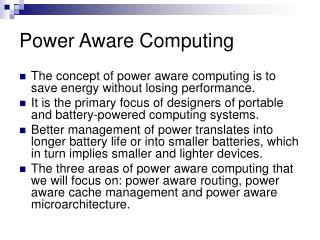
48. Power, energy, heat – oh, my • Relationship • E = P * T • H a E • Thus: control power • Goal • Conserve (reduce) energy consumption • Reduce heat generation • Regulate instantaneous power consumption • Situations (benefits) • Mobile/embedded computing (finite energy store) • Desktops (save $) • Servers, etc (increase performance)

49. Power usage • CPU power • Dominated by dynamic power • System power dominated by • CPU • Disk • Memory • CPU notes • Scalable • Driver of other system • Measure of performance power performance (freq) CMOS dynamic power equation: P = ½CfV2

50. Power management in HPC • Goals • Reduce heat generation (and $) • Increase performance • Mechanisms • Scaling • Feedback • Load balancing