Examples of Spatial Patterns

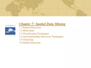
1. Chapter 7: Spatial Data Mining7.1 Pattern Discovery7.2 Motivation7.3 Classification Techniques7.4 Association Rule Discovery Techniques7.5 Clustering7.6 Outlier Detection

2. Examples of Spatial Patterns • Historic Examples (section 7.1.5, pp.186) • 1855 Asiatic Cholera in London : a water pump identified as the source • Fluoride and healthy gums near Colorado river • Theory of Gondwanaland - continents fit like pieces of a jigsaw puzzle • Modern Examples • Cancer clusters to investigate environment health hazards • Crime hotspots for planning police patrol routes • Bald eagles nest on tall trees near open water • Nile virus spreading from north east USA to south and west • Unusual warming of Pacific ocean (El Nino) affects weather in USA

3. What is a Spatial Pattern ? • What is not a pattern? • Random, haphazard, chance, stray, accidental, unexpected • Without definite direction, trend, rule, method, design, aim, purpose • Accidental - without design, outside regular course of things • Casual - absence of pre-arrangement, relatively unimportant • Fortuitous - What occurs without known cause • What is a Pattern? • A frequent arrangement, configuration, composition, regularity • A rule, law, method, design, description • A major direction, trend, prediction • A significant surface irregularity or unevenness

4. What is Spatial Data Mining? • Metaphors • Mining nuggets of information embedded in large databases • nuggets = interesting, useful, unexpected spatial patterns • mining = looking for nuggets • Needle in a haystack • Defining Spatial Data Mining • Search for spatial patterns • Non-trivial search - as “automated” as possible—reduce human effort • Interesting, useful and unexpected spatial pattern

5. What is Spatial Data Mining? - 2 • Non-trivial search for interesting and unexpected spatial pattern • Non-trivial Search • Large (e.g. exponential) search space of plausible hypothesis • Example - Figure 7.2, pp.186 • Ex. Asiatic cholera : causes: water, food, air, insects, …; water delivery mechanisms - numerous pumps, rivers, ponds, wells, pipes, ... • Interesting • Useful in certain application domain • Ex. Shutting off identified Water pump => saved human life • Unexpected • Pattern is not common knowledge • May provide a new understanding of world • Ex. Water pump - Cholera connection lead to the “germ” theory

6. What is NOT Spatial Data Mining? • Simple Querying of Spatial Data • Find neighbors of Canada given names and boundaries of all countries • Find shortest path from Boston to Houston in a freeway map • Search space is not large (not exponential) • Testing a hypothesis via a primary data analysis • Ex. Female chimpanzee territories are smaller than male territories • Search space is not large ! • SDM: secondary data analysis to generate multiple plausible hypotheses • Uninteresting or obvious patterns in spatial data • Heavy rainfall in Minneapolis is correlated with heavy rainfall in St. Paul, Given that the two cities are 10 miles apart. • Common knowledge: Nearby places have similar rainfall • Mining of non-spatial data • Diaper sales and beer sales are correlated in evenings • GPS product buyers are of 3 kinds: • outdoors enthusiasts, farmers, technology enthusiasts

7. Why Learn about Spatial Data Mining? • Two basic reasons for new work • Consideration of use in certain application domains • Provide fundamental new understanding • Application domains • Scale up secondary spatial (statistical) analysis to very large datasets • describe/explain locations of human settlements in last 5000 years • find cancer clusters to locate hazardous environments • prepare land-use maps from satellite imagery • predict habitat suitable for endangered species • Find new spatial patterns • find groups of co-located geographic features • Exercise. Name 2 application domains not listed above.

8. Why Learn about Spatial Data Mining? - 2 • New understanding of geographic processes for Critical questions • Ex. How is the health of planet Earth? • Ex. Characterize effects of human activity on environment and ecology • Ex. Predict effect of El Nino on weather, and economy • Traditional approach: manually generate and test hypothesis • But, spatial data is growing too fast to analyze manually • satellite imagery, GPS tracks, sensors on highways, … • Number of possible geographic hypothesis too large to explore manually • large number of geographic features and locations • number of interacting subsets of features grow exponentially • ex. find tele-connections between weather events across ocean and land areas • SDM may reduce the set of plausible hypothesis • Identify hypothesis supported by the data • For further exploration using traditional statistical methods

9. Spatial Data Mining: Actors • Domain Expert - • Identifies SDM goals, spatial dataset, • Describe domain knowledge, e.g. well-known patterns, e.g. correlates • Validation of new patterns • Data Mining Analyst • Helps identify pattern families, SDM techniques to be used • Explain the SDM outputs to Domain Expert • Joint effort • Feature selection • Selection of patterns for further exploration

10. The Data Mining Process Figure 7.1

11. Choice of Methods • 2 Approaches to mining Spatial Data • Pick spatial features; use classical DM methods • Use novel spatial data mining techniques • Possible Approach: • Define the problem: capture special needs • Explore data using maps, other visualization • Try reusing classical DM methods • If classical DM perform poorly, try new methods • Evaluate chosen methods rigorously • Performance tuning as needed

12. Families of SDM Patterns • Common families of spatial patterns • Location Prediction: Where will a phenomenon occur ? • Spatial Interaction: Which subsets of spatial phenomena interact? • Hot spots: Which locations are unusual ? • Note: • Other families of spatial patterns may be defined • SDM is a growing field, which should accommodate new pattern families

13. Location Prediction • Question addressed • Where will a phenomenon occur? • Which spatial events are predictable? • How can a spatial events be predicted from other spatial events? • equations, rules, other methods, • Examples: • Where will an endangered bird nest ? • Which areas are prone to fire given maps of vegetation, draught, etc.? • What should be recommended to a traveler in a given location? • Exercise: • List two prediction patterns.

14. Spatial Interactions • Question addressed • Which spatial events are related to each other? • Which spatial phenomena depend on other phenomenon? • Examples: • Exercise: List two interaction patterns

15. Hot spots • Question addressed • Is a phenomenon spatially clustered? • Which spatial entities or clusters are unusual? • Which spatial entities share common characteristics? • Examples: • Cancer clusters [CDC] to launch investigations • Crime hot spots to plan police patrols • Defining unusual • Comparison group: • neighborhood • entire population • Significance: probability of being unusual is high

16. Categorizing Families of SDM Patterns • Recall spatial data model concepts from Chapter 2 • Entities - Categories of distinct, identifiable, relevant things • Attribute: Properties, features, or characteristics of entities • Instance of an entity - individual occurrence of entities • Relationship: interactions or connection among entities, e.g. neighbor • Degree - number of participating entities • Cardinality - number of instance of an entity in an instance of relationship • Self-referencing - interaction among instance of a single entity • Instance of a relationship - individual occurrence of relationships • Pattern families (PF) in entity relationship models • Relationships among entities, e.g. neighbor • Value-based interactions among attributes, • e.g. Value of Student.age is determined by Student.date-of-birth

17. Families of SDM Patterns • Common families of spatial patterns • Location Prediction: • determination of value of a special attribute of an entity is by values of other attributes of the same entity • Spatial Interaction: • N-ry interaction among subsets of entities • N-ry interactions among categorical attributes of an entity • Hot spots: self-referencing interaction among instances of an entity • ... • Note: • Other families of spatial patterns may be defined • SDM is a growing field, which should accommodate new pattern families

18. Unique Properties of Spatial Patterns • Items in a traditional data are independent of each other, • whereas properties of locations in a map are often “auto-correlated” • Traditional data deals with simple domains, e.g. numbers and symbols, • whereas spatial data types are complex • Items in traditional data describe discrete objects • whereas spatial data is continuous • First law of geography [Tobler]: • Everything is related to everything, but nearby things are more related than distant things. • People with similar backgrounds tend to live in the same area • Economies of nearby regions tend to be similar • Changes in temperature occur gradually over space (and time)

19. Example: Clustering and Auto-correlation • Note clustering of nest sites and smooth variation of spatial attributes (Figure 7.3, pp.188 includes maps of two other attributes) • Also see Figure 7.4 (pp.189) for distributions with no autocorrelation

20. Moran’s I: a Measure of Spatial Autocorrelation • Given sampled over n locations. Moran I is defined as where and W is a normalized contiguity matrix Figure 7.5

21. Moran I - example Figure 7.5 • Pixel value set in (b) and (c ) are same Moran I is different. • Q? Which dataset between (b) and (c) has higher spatial autocorrelation?

22. Basic of Probability Calculus • Given a set of events , the probability P is a function from into [0,1] which satisfies the following two axioms • and • If A and B are mutually exclusive events then P(AB) = P(A)P(B) • Conditional Probability: • Given that an event B has occurred the conditional probability that event A will occur is P(A|B). A basic rule is • P(AB) = P(A|B)P(B) = P(B|A)P(A) • Baye’s rule: allows inversions of probabilities • Well known regression equation • allows derivation of linear models

23. Mapping Techniques to Spatial Pattern Families • Overview • There are many techniques to find a spatial pattern family • Choice of technique depends on feature selection, spatial data, etc. • Spatial pattern families vs. techniques • Location Prediction: Classification, function determination • Interaction : Correlation, Association, Colocations • Hot spots: Clustering, Outlier Detection • We discuss these techniques now • With emphasis on spatial problems • Even though these techniques apply to non-spatial datasets too

24. Location Prediction as a Classification Problem Given: 1. Spatial Framework 2. Explanatory functions: 3. A dependent class: 4. A family of function mappings: Find:Classification model: Objective: maximizeclassification accuracy Constraints: Spatial Autocorrelation exists Nest locations Distance to open water Vegetation durability Water depth Color version of Figure 7.3

25. Techniques for Location Prediction • Classical method: • Logistic regression, decision trees, Bayesian classifier • Assumes learning samples are independent of each other • Spatial auto-correlation violates this assumption! • Q? What will a map look like where the properties of a pixel was independent of the properties of other pixels? (see below Figure 7.4) • New spatial methods • Spatial auto-regression (SAR) • Markov random field • Bayesian classifier

26. Spatial Auto-Regression (SAR) • Spatial Auto-regression Model (SAR) • y = Wy + X +  • W models neighborhood relationships •  models strength of spatial dependencies •  error vector • Solutions •  and  - can be estimated using ML or Bayesian stat • e.g., spatial econometrics package uses Bayesian approach using sampling-based Markov Chain Monte Carlo (MCMC) method • likelihood-based estimation requires O(n3) ops • other alternatives – divide and conquer, sparse matrix, LU decomposition, etc.

27. Model Evaluation • Confusion matrix M for 2 class problems • 2 Rows: actual nest (True), actual non-nest (False) • 2 Columns: predicted nests (Positive), predicted non-nest (Negative) • 4 cells listing number of pixels in following groups • Figure 7.7 (pp.196) • nest is correctly predicted – (True Positive TP) • model can predict nest where there was none – (False Positive FP) • no-nest is correctly classified - (True Negative TN) • no-nest is predicted at a nest - (False Negative FN)

28. Model Evaluation continued • Outcomes of classification algorithms are typically probabilities • Probabilities are converted to class-labels by choosing a threshold level b. • For example probability >b is “nest” and probability <b is `no-nest’ • TPR is the True Positive Rate, FPR is the False Positive Rate

29. Comparing Linear and Spatial Regression • The further the curve away from the line TPR=FPR the better • SAR provides better predictions than regression model (Figure 7.8)

30. MRF Bayesian Classifier • Markov Random Field based Bayesian Classifiers • Pr(li | X, Li) = Pr(X|li, Li) Pr(li | Li) / Pr (X) • Pr(li | Li) can be estimated from training data • Li denotes set of labels in the neighborhood of si excluding labels at si • Pr(X|li, Li) can be estimated using kernel functions • Solutions • stochastic relaxation [Geman] • Iterated conditional modes [Besag] • Graph cut [Boykov]

31. Comparison (MRF-BC vs. SAR) • SAR can be rewritten as y = (QX)  + Q • where Q = (I- W)-1, a spatial transform. • SAR assumes linear separability of classes in transformed feature space • MRF model may yields better classification accuracies than SAR, • if classes are not linearly separable in transformed space • The relationship between SAR and MRF are analogous to the relationship between logistic regression and Bayesian classifiers

32. MRF vs. SAR (Summary)

33. Techniques for Association Mining • Classical method: • Association rule given item-types and transactions • Assumes spatial data can be decomposed into transactions • However, such decomposition may alter spatial patterns • New spatial methods • Spatial association rules • Spatial co-locations • Note: Association rule or co-location rules are fast filters to reduce the number of pairs for rigorous statistical analysis, e.g. correlation analysis, cross-K-function for spatial interaction etc. • Motivating example - next slide

34. Associations, Spatial associations, Co-location Answers: and Find patterns from the following sample dataset?

35. Colocation Rules – Spatial Interest Measures

36. Association Rules Discovery • Association rules has three parts • Rule: XY or antecedent (X) implies consequent (Y) • Support = the number of time a rule shows up in a database • Confidence = Conditional probability of Y given X • Examples • Generic - Diaper-beer sell together weekday evenings [Walmart] • Spatial: • (bedrock type = limestone), (soil depth < 50 feet) => (sink hole risk = high) • support = 20 percent, confidence = 0.8 • interpretation: Locations with limestone bedrock and low soil depth have high risk of sink hole formation.

37. Association Rules: Formal Definitions • Consider a set of items, • Consider a set of transactions • where each is a subset of I. • Support of C • Then iff • Support: occurs in at least s percent of the transactions: • Confidence: at least c% • Example: Table 7.4 (pp. 202) using data in Section 7.4

38. Apriori Algorithm to Mine Association Rules • Key challenge • Very large search space • N item-types => power(2,N) possible associations • Key assumption • Few associations are support above given threshold • Associations with low support are not intresting • Key Insight - Monotonicity • If an association item set has high support, ten so do all its subsets • Details • Psuedo code on pp.203 • Execution trace example - Figure 7.11 on next slide

39. Association Rules: Example

40. Spatial Association Rules • Spatial Association Rules • A special reference spatial feature • Transactions are defined around instance of special spatial feature • Item-types = spatial predicates • Example: Table 7.5 (pp.204)

41. Colocation Rules • Motivation • Association rules need transactions (subsets of instance of item-types) • Spatial data is continuous • Decomposing spatial data into transactions may alter patterns • Co-location Rules • For point data in space • Does not need transaction, works directly with continuous space • Use neighborhood definition and spatial joins • “Natural approach”

42. Colocation Rules

43. Association rules Co-location rules Underlying space discrete sets continuous space item-types item-types events /Boolean spatial features collection Transaction (T) Neighborhood (N) prevalence measure support participation index conditional probability metric Pr.[ A in T | B in T ] Pr.[ A in N(L) | B at location L ] Co-location rules vs. Association Rules Participation index = min{pr(fi,c)} where pr(fi,c) of feature fi in co-location c = {f1,f2,…,fk}: = fraction of instances of fi with feature {f1,…,fi-1,fi+1,…,fk} nearby N(L) = neighborhood of location L

44. Idea of Clustering • Clustering • Process of discovering groups in large databases. • Spatial view: rows in a database = points in a multi-dimensional space • Visualization may reveal interesting groups • A diverse family of techniques based on available group descriptions • Example: census 2001 • Attribute based groups • homogeneous groups, e.g. urban core, suburbs, rural • central places or major population centers • hierarchical groups: NE corridor, Metropolitan area, major cities, neighborhoods • areas with unusually high population growth/decline • Purpose based groups, e.g. segment population by consumer behavior • data driven grouping with little a priori description of groups • many different ways of grouping using age, income, spending, ethnicity, ...

45. Spatial Clustering Example • Example data: population density • Figure 7.13 (pp.207) on next slide • Grouping Goal - central places • Identify locations that dominate surroundings • Groups are S1 and S2 • Grouping goal - homogeneous areas • Groups are A1 and A2 • Note: Clustering literature may not identify the grouping goals explicitly • Such clustering methods may be used for purpose based group finding

46. Spatial Clustering Example • Example data: population density • Figure 7.13 (pp.207) • Grouping Goal - central places • Identify locations that dominate surroundings, • Groups are S1 and S2 • Grouping goal - homogeneous areas • Groups are A1 and A2

47. Spatial Clustering Example Figure 7.13

48. Techniques for Clustering • Categorizing classical methods: • Hierarchical methods • Partitioning methods, e.g. K-mean, K-medoid • Density based methods • Grid based methods • New spatial methods • Comparison with complete spatial random processes • Neighborhood EM • Our focus: • Section 7.5: Partitioning methods and new spatial methods • Section 7.6 on outlier detection has methods similar to density based methods

49. Algorithmic Ideas in Clustering • Hierarchical— • All points in one clusters • Then splits and merges till a stopping criterion is reached • Partitional— • Start with random central points • Assign points to nearest central point • Update the central points • Approach with statistical rigor • Density • Find clusters based on density of regions • Grid-based— • Quantize the clustering space into finite number of cells • Use thresholding to pick high density cells • Merge neighboring cells to form clusters

50. Idea of Outliers • What is an outlier? • Observations inconsistent with rest of the dataset • Ex. Point D, L or G in Figure 7.16(a), pp.216 • Techniques for global outliers • Statistical tests based on membership in a distribution • Pr.[item in population] is low • Non-statistical tests based on distance, nearest neighbors, convex hull, etc. • What is a special outliers? • Observations inconsistent with their neighborhoods • A local instability or discontinuity • Ex. Point S in Figure 7.16(a), pp. 216 • New techniques for spatial outliers • Graphical - Variogram cloud, Moran scatterplot • Algebraic - Scatterplot, Z(S(x))