DATA VISUALIZATION
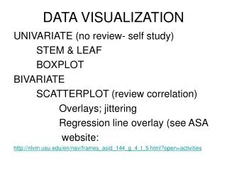
DATA VISUALIZATION. UNIVARIATE (no review- self study) STEM & LEAF BOXPLOT BIVARIATE SCATTERPLOT (review correlation) Overlays; jittering Regression line overlay (see ASA website: http://nlvm.usu.edu/en/nav/frames_asid_144_g_4_t_5.html?open=activities. DATA VISUALIZATION.

DATA VISUALIZATION
E N D
Presentation Transcript
DATA VISUALIZATION UNIVARIATE (no review- self study) STEM & LEAF BOXPLOT BIVARIATE SCATTERPLOT (review correlation) Overlays; jittering Regression line overlay (see ASA website: http://nlvm.usu.edu/en/nav/frames_asid_144_g_4_t_5.html?open=activities
DATA VISUALIZATION TOPICS GRAPHICAL DISPLAYS UNIVARIATE BIVARIATE ASSUMPTIONS OF MULTIPLE REGRESSION LINEARITY HOMOSCEDASTICITY ERROR INDEPENDENCE NORMALITY FIXING VIOLATIONS
GRAPHICAL DISPLAYS • Frequency Histogram: • SPSS ANALYZE: Descriptive Statistics: Explore: Plot: Stem and Leaf • SPSS GRAPH: Boxplot (normal curve overlay available • or INTERACTIVE: Boxplot or Analyze: Frequencies • SPSS GRAPH: Histogram or Interactive: Histogram • # “bins” = 1 + log2(N) • Example: N= 500; #bins = 1+ 9 = 10 • Log2(512) = 9 (eg., 2x2x2x2x2x2x2x2x2=512)
ANXIETY Stem-and-Leaf Plot Frequency Stem & Leaf .00 3 . 22.00 3 . 4444444444455555555555 35.00 3 . 66666666777777777777777777777777777 7.00 3 . 9999999 39.00 4 . 000000000000000000000000011111111111111 22.00 4 . 2222222222222222222222 26.00 4 . 44455555555555555555555555 22.00 4 . 6666666667777777777777 26.00 4 . 88888888888999999999999999 12.00 5 . 111111111111 26.00 5 . 22222222222222222223333333 14.00 5 . 44444444444444 24.00 5 . 666666777777777777777777 31.00 5 . 8888888888888999999999999999999 28.00 6 . 1111111111111111111111111111 6.00 6 . 333333 15.00 6 . 444444444444444 24.00 6 . 666666666666666666666666 14.00 6 . 88888899999999 Stem width: 10 Each leaf: 1 case(s)
GRAPHICAL DISPLAYS • Kernel Smoothing • SPSS Graph: INTERACTIVE: Line: Dots and Lines: Spline or Lagrange 3rd and 5th order fits • does not give you the smoother options (available for bivariate scatterplots- see later slides)
Bivariate Displays • Scatterplots • Interval data • Category by interval- jittering • Regression fits- lowess lines • Scatterplot Matrices
Interval Scatterplot: SPSS Graphics: Interactive: Scatterplot: Fit: Method:Smoother No Smoother with Normal Smoother
Interval Scatterplot: SPSS Graphics: Interactive: Scatterplot: Fit: Method:Smoother with Uniform Smoother
Category X-axis: without and with jittering (adding normal random deviate with SD=.15 for sex)
Jittering • Basic idea- when looking at displays for two or more groups, it is hard to tell where data lie due to overlaying of points in most plot programs, so • Add a small random score to each “group” score • For example, for males (score 1) and females (score 2), add a random number with std dev. of say .1 to each male and female score
Jittering • The result is a spreading out of all scores around the Male or Female column in a scatterplot: . . . . . . . . . . . . . . . . Y Male=1 Female=2
DATA VISUALIZATION BIVARIATE Loess lines: in SPSS an option under GRAPH/ Interactive / Scatterplot labeled “FIT” with METHOD = SMOOTHER The Bandwidth multiplier has a 1.0 default; a smaller value will create more bumps or curves in the overall curve