Download
1 / 20
270 likes | 948 Vues
Lecture 5: Time-varying EM Fields. Instructor: Dr. Gleb V. Tcheslavski Contact: gleb@ee.lamar.edu Office Hours: Room 2030 Class web site: www.ee.lamar.edu/gleb/em/Index.htm. Introduction .

E N D
Lecture 5: Time-varying EM Fields Instructor: Dr. Gleb V. Tcheslavski Contact:gleb@ee.lamar.edu Office Hours: Room 2030 Class web site:www.ee.lamar.edu/gleb/em/Index.htm
Introduction Although “Time-varying EM fields” is the title of the present lecture only, the rest of our course will be devoted to time-varying fields! These fields are generalizations of electrostatic and magnetostatic fields studied earlier.
Faraday’s law of induction We consider an electric potential across an inductor inserted in a circuit. The voltage across the inductor can be expressed as (5.3.1) where L is the inductance [H], I(t) – time varying current passing through the inductor.
Faraday’s law of induction We have learned that a constant current induces magnetic field and a constant charge (or a voltage) makes an electric field. Similar phenomena happen when currents/voltages are changing in time. The relation between the electric and magnetic field components is governed by the Faraday’s law… (5.4.1) Lentz’s law where is the total time-varying magnetic flux passing through a surface. Voltage is induced in a closed loop that completely surrounds the surface, through which the magnetic flux passes.
Faraday’s law of induction Therefore, we consider an individual turn of a coil (inductor) as a closed loop. At a glance: an electric current (an emf) is generated in a closed loop when any change in magnetic environment around the loop occurs (Faraday’s law). When an emf is generated by a change in magnetic flux according to Faraday's Law, the polarity of the induced emf is such that it produces a current whose magnetic field opposes the change which produces it. The induced magnetic field inside any loop of wire always acts to keep the magnetic flux in the loop constant.
Faraday’s law of induction The total magnetic flux passing through the loop is (5.6.1) The terminals of the loop are separated by an infinitely small distance, therefore, we assume the loop as closed. Recall from (3.20.2) that the electric potential can be expressed as (5.6.2) Combining two last equations with (5.4.1) yields the integral form of Faraday’s law: (5.6.3)
Faraday’s law of induction Application of the Stokes’s theorem to the integral form of the Faraday’s law of induction leads to (5.7.1) Equality of integrals implies an equality of integrands, therefore: (5.7.2) Is a differential form of the Faraday’s law of induction.
Faraday’s law of induction (Ex) A good illustration of the Faraday’s law of induction is an ideal transformer. Find the voltage V2 at the loop 2 (secondary coil) if the voltage V1 is applied to the loop 1 (primary coil). The “ideal” assumption implies no loss in the core and that the core has infinite permeability. (5.8.1)
Faraday’s law of induction We assumed previously that the area of the loop s is not changing. It does not always hold. Let us consider a conductive bar moving at a speed v through a constant uniform magnetic field B. The Lorentz force will cause a charge separation within the conductor. Charge separation will create an electric field. Since the net force on the bar is zero, the electric and magnetic contributions must cancel each other. Therefore: (5.9.1) Electric field is an induced field acting along conductor and producing: (5.9.2)
Faraday’s law of induction Example: a Faraday’s disc generator consists of a metal disc rotating with a constant angular velocity = 600 1/s in a uniform time-independent magnetic field with a magnetic flux density B = B0uz, where B0 = 4 T. Determine the induced voltage generated between the brush contacts at the axis and the edge of the disc, whose radius a = 0.5 m. An electron at a radius from the center has a velocity . Therefore, the potential generated is: (5.10.1)
Faraday’s law of induction We can evaluate a divergence for both sides of the Faraday’s law: (5.11.1) Since divergence of the curl is zero: (5.11.2) Or in the integral form: (5.11.3) Same as for MS fields, there is no magnetic monopole and magnetic lines are continuous.
Equation of Continuity (5.12.1) Current density is the movement of charge density. The continuity equation says that if charge is moving out of a differential volume (i.e. divergence of current density is positive) then the amount of charge within that volume is going to decrease, so the rate of change of charge density is negative. Therefore the continuity equation amounts to a conservation of charge.
Equation of Continuity Example: charges are introduced into the interior of a conductor during the time t < 0. Calculate the time needed for charges to move to the surface of the conductor so the interior charge density v = 0 and interior electric field E = 0. Let us combine the Ohm’s law and the continuity equation: (5.13.1) The Poisson’s equation: (5.13.2) Therefore: (5.13.3) The solution will be: (5.13.4)
Equation of Continuity The initial charge density v decays to 1/e 37% of its initial value in a relaxation time = /. (5.14.1) For copper, the relaxation time is: (5.14.2) For dielectric materials, the relaxation time can be quite big: hours or even days.
Displacement current Maxwell’s experiment: Connect together an AC voltage source, an AC ammeter reading a constant current I and an ideal parallel plate capacitor… • How can the ammeter read any values if the capacitor is an open circuit? • What happens to the time-varying magnetic field that is created by the current and surrounds the wire as we pass through the vacuum between the capacitor’s plates? The Ampere’s law: (5.15.1)
Displacement current Applying the divergence operation to both sides of the Ampere’s law, we get: (5.16.1) (5.16.2) and However, the last expression disagrees with the equation of continuity… To overcome this contradiction, we introduce an additional current called a displacement current, whose current density will be Jd. The continuity equation: (5.16.2)
Displacement current Therefore, the displacement current density is: (5.17.1) This is the current passing between the plates of the capacitor. As a consequence, the postulate of Magnetostatic we discussed previously must be modified as follows: Differential form: (5.17.2) Integral form: (5.17.3)
Displacement current Example 1: Verify that the conduction current in the wire equals to the displacement current between the plates of the parallel plate capacitor in Figure. The voltage source supplies: Vc = V0 sin t. (5.18.1) The conduction current in the wire is (5.18.2) The capacitance of a parallel plate capacitor is: (5.18.3) The electric field between the plates: (5.18.4) The displacement flux density is: (5.18.5) Finally: (5.18.6)
Displacement current Example 2: Find the displacement current, the displacement charge density, and the volume charge density associated with the magnetic flux density in a vacuum: (5.19.1) There is no conductors, therefore, only the displacement flux exists. (5.19.2) The displacement flux density: (5.19.3) From the Gauss’s law: (5.19.4)
Displacement current Example 3: In a lossy dielectric with a conductivity and a relative permittivity r, there is a time-harmonic electric field E = E0sin t. Compare the magnitudes of the conduction current density and the displacement current density. Conduction current density: Displacement current density: The ratio of the magnitudes is: HW 4 is ready.