Download
1 / 52
550 likes | 1.03k Vues
USGS. science for a changing world. Modeling Ground Water Interactions with Surface Water. Western States Water Council . Water Information Management Systems Meeting Albuquerque, New Mexico September 13, 2006. David E. Prudic U.S. Geological Survey Carson City, Nevada. USGS.

E N D
USGS science for a changing world Modeling Ground Water Interactions with Surface Water Western States Water Council Water Information Management Systems MeetingAlbuquerque, New Mexico September 13, 2006 David E. PrudicU.S. Geological SurveyCarson City, Nevada
USGS science for a changing world “When the well’s dry, we know the worth of water” Benjamin Franklin Add “streams” and this statement embodies the history of development in the Western United States during the past two centuries
USGS science for a changing world Ground-Water Interactions with Surface Water is Ever Changing Modeling ground-water interactions with surface water is difficult because of variability in climate, and changing practices in the development of surface-water and ground-water supplies
USGS science for a changing world History of Development Knowing the history of an area is key to understanding and modeling ground water interactions with surface water
USGS science for a changing world Development is Divided into Three Periods • Local diversion of water from streams for mining and irrigation of areas in adjacent flood plains • Development of large reservoirs and complex irrigation systems for areas distant from the flood plains • Development of deep turbine pumps and pivot irrigation systems for ground-water irrigation
USGS science for a changing world First Period • Excess diversion of streams led to the development of laws and the Doctrine of Prior Appropriation • Decreased annual stream flow • Raised ground-water levels and increased ground-water discharge to streams during periods of low flow
USGS science for a changing world Second Period • Development of a “Concentrated Hydraulic Society” to utilize and maintain infrastructure • Decreased annual flows of streams • Increased ground water in storage around reservoirs • Increased ground-water levels (storage) in areas distant from rivers • Localized water logging, creation of wetlands, and construction of drains • Increased diffuse ground-water discharge to evapotranspiration near areas of irrigation
USGS science for a changing world Third Period • Development of a “Distributed Hydraulic Society” from the drilling and pumping of thousands of individual wells with minimum regulation • Decreased ground-water levels and storage • Decrease in streamflows slow to develop because of large ground-water storage capacity
USGS science for a changing world Modeling Ground-Water and Surface Water Interaction Modeling approach traditionally has depended on perspective—one either asked: • How does surface water influence ground-water flow? or • How does ground water influence the surface-water flow? S. A. Leake
USGS science for a changing world Surface-Water Hydraulics Simulation Model Black Box Groundwater S. A. Leake
USGS science for a changing world Ground-Water Flow Model Surface-water processes S. A. Leake
USGS science for a changing world Numerical Simulation of Surface Water and Ground Water Interaction Many questions regarding effects of ground-water withdrawals on surface water are difficult to answer because: • Aquifers that interact with surface water are often heterogeneous and • Both surface-water and ground-water flows can change in time and space
Darcy’s Law: Infinitesimal volume of aquifer USGS science for a changing world Ground-Water Flow Equation The equation is simply an expression of mass balance S. A. Leake
Infinitesimal volume of aquifer USGS science for a changing world Ground-Water Flow Equation, “W” term The “W” term is flow rate per unit volume of aquifer added to or taken from ground-water system. Q3 Q1 Q2 Most interaction between ground water and surface water is lumped into the W term S. A. Leake
USGS science for a changing world Common types of surface-water boundaries in ground-water models: • “Constant” or “specified” flow • “Constant” or “specified” head • Head-dependent flow— Q = f(h)May be reasonable for large lakes and rivers not affected by changes in ground-water flow because quantity of surface water is not part of calculation S. A. Leake
Q1 Q2 Q3 Q4 Q6 USGS Q5 science for a changing world Constant or specified flow boundaries • Flow rate is specified in model grid cell as known value of recharge or discharge • Model computes head at boundary location Example: Divide total streamflow loss or gain into parts belonging in each cell NOTE: Make sure model-computed head is reasonable at these locations! S. A. Leake
h1 h2 h3 h4 h6 USGS h5 science for a changing world Constant or specified head boundaries • Head in model grid cell corresponding to surface-water location is specified as elevation of water surface • Flow rate to or from boundary is computed from adjacent model grid cells • Does not require a “W” term in flow equation Example: Determine average stream stage in each cell traversed by stream. Assign stage values as specified head in cells. NOTE: Make sure model-computed flow is reasonable at these locations! S. A. Leake
USGS science for a changing world Head-dependent flow boundaries: • A functional relationship between head in aquifer and flow to or from boundary is derived, usually by Darcy’s law • Function is made part of “W” term • Most model programs, such as MODFLOW have several such functions built in • The ground-water head now occurs in the “W” term, possibly adding difficulty to the solution S. A. Leake
USGS science for a changing world Ground-water model “Real world” Streambed sediments Cross section: Head in stream Head in cell Plan view: Area of stream Area encompassed by model cell Model cell S. A. Leake
USGS science for a changing world Ground-water model Head in stream Head in cell Idealized prism of river bed sediments contained in a model cell Model cell S. A. Leake
USGS science for a changing world Flow Through Streambed An expression of flow through the streambed is computed from Darcy’s Law as: Head here is river head, HRIV Length, L Head here is aquifer head, HAQ Width, W Thickness, b Vertical hydraulic conductivity is, Kv Q = Csfr (HSTR-HAQ) where Csfr = Kv (LW)/b S. A. Leake
USGS science for a changing world Routing of Surface Water • Surface routing programs are used to simulate changing location of flow and recharge to an aquifer without having to manually specify stage or flow in every reach • Stage and streambed conductance term can vary in relation to channel dimensions and flow
USGS science for a changing world Typical Method of Routing Streamflows Section 1 Flow direction Section 2 Section 5 Section 3 Section 6 Section 4 SQin = SQout+DStorage
USGS science for a changing world Three Surface-Water Routing Programs Connected to MODFLOW • Streamflow-Routing Package (STR1) recently rewritten (SFR1 & SFR2) to include different flow options, solute transport, and unsaturated flow—Myself and others (1989; 2004 and 2005) • Diffusion Analogy Surface-Water Flow Model (DAFLOW) – Harvey Jobson, USGS Open-file Report 99-217 • Branch Surface-Water Flow Model (MODBRANCH)– Eric Swain and E. J. Wexler, USGS TWRI Book 6, Chapter A6
USGS science for a changing world Streamflow-Routing Package (STR1, SFR1, and SFR2) • Simple routing through network of streams assuming no change in storage and sum of inflow equals outflow • Stream depth computed using different options assuming steady, uniform flow Upstream flow Precipitation OverlandRunoff ET Downstream flow Leakage
USGS science for a changing world DAFLOW Continuity of Mass • One-dimensional unsteady flow in network of open channels • Solves equations for continuity of mass and momentum assuming no lateral inflow • Approximates flow in a stream as reaches of steady uniform flow separated by transitions of unsteady flow Continuity of Momentum Q is discharge, U is velocity, A is cross-section area, t is time L is channel Length, y is depth, G is acceleration of gravity, Sf is friction slope, and So is streambed slope
USGS science for a changing world DAFLOW Transitionof unsteady flow Steady flow Flow Control volume t Q2, A2 t + Dt Friction slopeat timet Steady flow Q1, A1 DL So So Flow into and out of control volume: , and where Cis speed of moving wave
USGS science for a changing world ModBranch • Combines one-dimensional unsteady flow model with MODFLOW • Solves equations for continuity of mass and momentum and allows lateral inflow and outflow (known as St. Venant equations) • Approximates changes in streamflow through finite-difference methods
USGS science for a changing world Stream Network Model rows Inflow Segment 1 Diversion Inflow Segment 3 Canal Segment 2 Point diversion Model columns Segment 5 Segment 4 Pipeline Segment junction Segment 6 Segment 7 Outflow
Joining reaches Parallel reaches 1 2 1 2 3 1 2 3 USGS science for a changing world Stream Reaches in a Cell • Flow into and out of each reach calculated during every MODFLOW iteration • Multiple stream reaches simulated for a model cell • Does not simulate multiple model cells for one stream reach GW node Only one cell per reach
USGS science for a changing world Inflow to a Reach Pipeline Tributary stream Flood wave Surface runoff Soil zone Interflow Water table Precipitation Ground-water discharge Finite-difference cell
USGS science for a changing world Outflow from a Reach Pipeline Flood wave Evaporation Diversion Streamflow out Stream leakage Stream leakage Finite-difference cell
USGS science for a changing world Diverting Flow into a Segment • Specified diversion • Diversion rate reduce to available flow • Diversion rate reset to zero when available flow less than specified diversion • Specified flow fraction available in stream • Flow diverted only when available flow exceeds a specified flow rate Last two options originally program by Randy Hanson, San Diego Office
USGS science for a changing world Stream Depth • Stream depth is computed at midpoint of each stream reach • Flow is computed at midpoint prior to computing stream depth except when a constant depth is specified Cell node Reachmidpoint Q = QIn + 0.5[Overland flow+(P*L*w)] -0.5[(ET*L*w)+leakage to GW]
USGS science for a changing world Stream Depth • Flow at midpoint is partly dependent on streambed leakage, which is dependent on stream depth that is dependent on flow • Equation is repeatedly solved using Newton’s method until • Change in stream stage is less than a specified value usually 0.0001 or • Average of last two stream stages after reaching a maximum of 50 iterations
USGS science for a changing world Options for Computing Stream DepthManning’s Equation for Wide Rectangular Channel Q = (C/n) A R2/3 S1/2 where A = area of rectangular channel (width * depth) R = hydraulic radius = Area divided by wetted perimeter R = depth when width (w) >>depth) C = constant (1.0 for m3/s and 1.486 for ft3/s) n = Manning’s roughness coefficient, dimensionless Depth can be computed as: d = [(Q/n)/(CwS 1/2)]3/5
USGS science for a changing world Eight Point Cross Section The eight point cross section is divided into three parts. Vertical walls are assumed at the end of each cross section Channel Left bank Right bank Part 2 Width Depth Wetted perimeter Depth, wetted perimeter, and width computed from cross section given flow.
USGS science for a changing world Log-Log equation The width (w), mean depth (d), and mean velocity (v) each increase with respect to discharge (Q) as power functions (Leopold, Wolman and Miller, 1964 and 1992, Fluvial Processes in Geomorphology) : WIDTH = aQb, DEPTH = cQf,VELOCITY = kQm wherea,b, c,f,k,andmare numerical coefficients becausew * d * v = Q;aQb*cQf *kQm = Q andb + f + m =1; anda * c * k = 1
USGS science for a changing world Depth Computed from Table • Table of depth and width versus flow is entered from data collected at a streamflow gage • Program uses log interpolation between values except when computed flow is between 0 and first value in table Flow Depth Width 5 10 0.5 50 1.3 15 100 1.8 20 1,000 2.6 35
USGS science for a changing world Different Options can be used for Each Stream Segment Wide rectangular channel Diversion canal - constant Table Eight-point cross section Log-log equation
Stream Basin Fill Bedrock USGS science for a changing world Simulation of Unsaturated Flow Beneath Streams • Details published in USGS Techniques and Methods 6A-13 (Niswonger and Prudic, 2005)
USGS science for a changing world Simulating Vertical Unsaturated Flow Beneath Streams (SFR2) • Formulation is based on kinematic wave solution to Richards’ equation (Smith, 1983) - Avoid instabilities associated with conventional unsaturated flow models - Speeds up computational time for applications to large basin scale simulations
USGS science for a changing world Infiltration Time Water Content Depth Time 1 Time 2 Time 3
USGS science for a changing world Unsaturated Zone Divided into Compartments Stream High stage 6 Streambed Depth, meters Normal stage 0 Unsaturated zonecompartment 0 14 Width, meters
USGS science for a changing world Ground Water Interactions with Lakes are Simulated Using the Lake Package (Merritt and Konikow, 2000) Pipeline Tributary stream Outlet stream Surface runoff Evaporation Interflow Precipitation Lake cell Ground-waterdischarge Lakebed Lake leakage Aquifer cell with node
USGS science for a changing world Connection of Streams with a Lake Model rows Segment 1 1 1 2 Segment 2 2 3 4 3 6 5 5 4 6 7 7 Lake 1 Model columns 8 9 1 2 3 4 5 Segment3
USGS science for a changing world Lake surface Lake bottom Lakebed thickness Lakebed Conductance terms Distance from base of lakebed to point in aquifer Aquifer Cross-sectional area Point in aquifer
USGS science for a changing world Lakes can Divide and Merge High stage—one lake, one water budget Lake Surface Saturated zone Low stage—two or more lakes with different water budgets Lake 2 Lake 1 Saturated zone
USGS science for a changing world Integration of PRMS with MODFLOW—GSFLOW, Version 1.0 Soil Zone in PRMS Streams and Lakes Interflow Soil-Moisture Dependent Flow Surfacerunoff Ground-water discharge Ground-water discharge Head-DependentFlow Soil-Moisture/Head-Dependent Flow Gravity drainagethrough unsaturated zone Leakage Ground water
USGS science for a changing world Hydrologic Response Units and Finite-Difference Grid, Sagehen Creek, Truckee, California