Hydrological Modeling
Hydrological Modeling. FISH 513 April 10, 2002. Overview:. What is wrong with simple statistical regressions of hydrologic response on impervious area? Toward a more complete understanding of normal flows. Distributed Hydrological Modeling

Hydrological Modeling
E N D
Presentation Transcript
Hydrological Modeling FISH 513 April 10, 2002
Overview: What is wrong with simple statistical regressions of hydrologic response on impervious area? Toward a more complete understanding of normal flows. Distributed Hydrological Modeling Example from applications of Distributed Hydrological Modeling at UW Changes in impervious area. Changes in forest cover. Global Climate Change.
Typical Representation of Effect of Impervious Area on Runoff Coefficient 1 Runoff Coefficient 0 0 100% Percent Impervious Area
What we really want to know is: What is the change from normal? Previous graph is 100% correct for dry initial conditions. What if it has just rained nonstop for five days . . . Well that never happens around here?
Representation of Effect of Impervious Area on Runoff Coefficient for extremely wet initial conditions 1 Runoff Coefficient 0 0 1 Percent Impervious Area
Therefore, normal response depends: Static Variables: Land Cover Impervious Area, etc Dynamic Variables: Soil Moisture Precipitation Intensity Storm Duration, etc. Numerous Studies have shown decreased effects of land use Change as antecedent conditions become wetter. Our task is to build a predictive model of what is normal… And that can’t be done without considering interaction of meteorology with land cover changes
Land surface characterization required by DHSVM • Terrain - 150 m. aggregated from 10 m. resolution DEM • Land Cover - 19 classes aggregated from over 200 GAP classes • Soils - 3 layers aggregated from 13 layers (31 different classes); variable soil depth from 1-3 meters • Stream Network - based on 0.25 km2 source area
Calibration Location (Snoqualmie) Testing: Cedar • Calibration to two USGS sites • Split sample validation at over 60 sites • Parameters transfer extremely well to other watersheds without recalibration
Application of DHSVM to lower Cedar River Watershed to assess impacts of changes in impervious area on basin hydrology Taylor Creek (14 km2) 5% imperv. Madsen Creek (5.4 km2) 20% imperv. Fraction Impervious Area (1998) 100 % 75 % 50 % 25 % 0 %
DHSVM Calibration to determine baseline parameters. Taylor Creek (5% impervious area) CFS Feb 1991 Mar 1991 Apr 1991 May 1991 Test of Impervious Area Representation (no re-calibration) Madsen Creek (20% impervious area) CFS 0 20 40 60 80 100 120 4/1/91 4/4/91 4/7/91 4/10/91
Observed (1991): 120 cfs peak, 3.6 inches total runoff 1991 Land Cover (20 % imperv.): 115 cfs peak, 3.2 inches total runoff Old Growth Forest: 58 cfs peak, 2.3 inches total runoff 100 % increase in peak cfs 4/5/1991 4/15/1991 4/20/1991
100 80 60 40 20 5 4 3 2 1
2020’s Mean Winter Increase = 1.6 C 2040’s Mean Winter Increase = 2.4 C Predicted Change in Mean Monthly Temperature due to Increased Carbon Dioxide Levels (Mean of 4 GCM’s) 2020’s (w.r.t mid 20th century climate) 2040’s (w.r.t mid 20th century climate) Temperature Increase (degrees C)
Change In Temperature Change in Precipitation Methodology for Assessing Impacts of Climate Change on Watershed hydrology Observed Meteorology At Stations in and near Target Watershed Synthetic “Observed” Record: Talt=Tobs + Delta T Palt = Pobs*(Delta P) DHSVM SWE Reservoir Inflow
Drought Cedar River Watershed: Retrospective Analysis of Average Snow Water Equivalent Under Current and Altered Climates Current 2025 2045 Current Low Year Becomes . . . 2025/2045 Best Case Snow Water Equivalent (mm)
Effect of Climate Change on Mean Monthly Inflow (1988 to 1996) to Cedar Reservoir Current 2025 2045 Higher Winter Flows: Increased Precipitation Higher Freezing Level -> More Rain Snowmelt 126,000 acre-ft 90,000 acre-ft 78,000 acre-ft Monthly Inflow (meters) Month
GAP, 1991 Basins for which streamflow was simulated for each vegetation scenario. GAP, 1991 is based on a 1991 LandSat image. Band Harvest has a total clear-cut area identical to GAP, 1991 but concentrated in the transient snow zone (700-900 m). The control simulation is the historic vegetation coverage (based on GAP with all clear-cuts regrown). Historic Vegetation Band harvest
Effect of forest canopy removal, Snoqualmie River at Snoqualmie Falls, February 1996 event Hourly Precipitation (mm) Low elevation(<300 m) snow (mm SWE)