Download

1 / 28
280 likes | 454 Vues
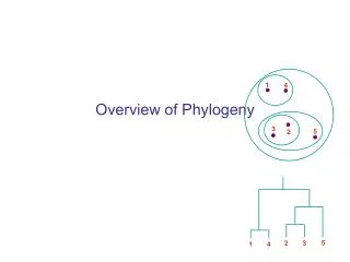
1. 4. 3. 5. 2. 5. 2. 3. 1. 4. Overview of Phylogeny. Edentata (anteaters, sloths, armadillos) . New World monkeys. Old World monkeys. Lagomorpha (rabbits) . humans, gorilla, chimpanzee, orangutan. Triconodonts. Rodentia (mice, rats, squirrels). gibbons. Multituberculata.

E N D
1 4 3 5 2 5 2 3 1 4 Overview of Phylogeny
Edentata (anteaters, sloths, armadillos) New World monkeys Old World monkeys Lagomorpha (rabbits) humans, gorilla, chimpanzee, orangutan Triconodonts Rodentia (mice, rats, squirrels) gibbons Multituberculata Mammals Primates Monotremata (platypus, echidnas) Tree shrews lemurs, galagos, lorises Bats Eutheria (placental animals) Colugos Artiodactyla (pigs, deer, cattle, goats, sheep, hippopotamuses, camels, etc.) Marsupialia (opossums, kangaroos) Cetacea (whales, dolphins, porpoises) Perissodactyla (horses, tapirs, rhinoceroses) Proboscidea (elephants, mammoths) Carnivora (dogs, cats, bears, raccons, weasels, mongooses, hyenas)
Phylogenies Phylogenies are trees that show the history of life Genes, repeats, etc., are also connected in phylogenies Orthologs: Two elements that have diverged because of speciation Paralogs: Two elements that have diverged because of duplication
Inferring Phylogenies Trees can be inferred: • Morphology of the organisms • Sequence comparison Example: Orc: ACAGTGACGCCCCAAACGT Elf: ACAGTGACGCTACAAACGT Dwarf: CCTGTGACGTAACAAACGA Hobbit: CCTGTGACGTAGCAAACGA Human: CCTGTGACGTAGCAAACGA
Background on trees root root 1 • Each node has three edges (binary) • Labeled • Each edge has a length (evolution time) • Unrooted, or rooted N leafs 2N – 2 nodes unrooted; 2N – 1 nodes rooted 4 12 8 3 13 7 9 5 11 10 6 2
Space of possible trees 1 1 1 1 unrooted tree of 3 leaves 3 unrooted trees of 4 leaves … 3 5 7 … (2N – 5) = (2N – 5)!! unrooted trees with N leaves (2N – 3)!! rooted trees with N leaves 4 1 4 4 3 2 3 2 3 2 2 3
Phylogeny and sequence comparison Basic principles: • Degree of sequence difference is proportional to length of independent sequence evolution • Only use positions where alignment is pretty certain – avoid areas with (too many) gaps
Distance between two sequences Given (portion of) sequences xi, xj, Define dij = distance between the two sequences One possible definition: dij = fraction f of sites u where xi[u] xj[u] Better model (Jukes-Cantor): dij = - ¾ log(1 – 4f / 3)
A simple clustering method for building tree UPGMA (unweighted pair group method using arithmetic averages) Given two disjoint clusters Ci, Cj of sequences, 1 dij = ––––––––– {p Ci, q Cj}dpq |Ci| |Cj| Note that if Ck = Ci Cj, then distance to another cluster Cl is: dil |Ci| + djl |Cj| dkl = –––––––––––––– |Ci| + |Cj|
Algorithm: UPGMA Initialization: Assign each xi into its own cluster Ci Define one leaf per sequence, height 0 Iteration: Find two clusters Ci, Cj s.t. dij is min Let Ck = Ci Cj Define node connecting Ci, Cj, height dij/2 Delete Ci, Cj Termination: When all sequences belong to one cluster 1 4 3 5 2 5 2 3 1 4
Ultrametric distances & UPGMA A distance measure is ultrametric if for any points i, j, k, Either all three distances are equal: dij = dik = djk, Or two of them are equal and one is smaller: djk < dij = dik UPGMA is guaranteed to build the correct tree if distance is ultrametric 5 2 3 1 4
Weakness of UPGMA Molecular clock: implied time is constant for all species However: certain species (e.g., mouse, rat) evolve much faster Example where UPGMA messes up: UPGMA Correct tree 3 2 1 3 4 4 2 1
Additivity of distance d1,4 1 Given a tree, a distance measure is additive if the distance between any pair of leaves is the sum of lengths of edges connecting them A maximum likelihood distance measure is additive given a large amount of data 4 12 8 3 13 7 9 5 11 10 6 2
Neighbor-joining • Guaranteed to produce the correct tree if distance is additive • May produce a good tree even when distance is not additive Step 1: Finding neighboring leaves Define Dij = dij – (ri + rj) Where 1 ri = –––––kdik |L| - 2 1 3 0.1 0.1 0.1 0.4 0.4 4 2
Algorithm: Neighbor-joining Initialization: Define T to be the set of leaf nodes, one per sequence Let L = T Iteration: Pick i, j s.t. Dij is minimal Define a new node k, and set dkm = ½ (dim + djm – dij) for all m L Add k to T, with edges of lengths dik = ½ (dij + ri – rj) Remove i, j from L; Add k to L Termination: When L consists of two nodes, i, j, and the edge between them of length dij
Rooting a tree, and definition of outgroup Neighbor-joining produces an unrooted tree How do we root a tree between N species using n-j? An outgroup is a species that we know to be more distantly related to all remaining species, than they are to one another Example: Human, mouse, rat, pig, dog, chicken, whale Which one is an outgroup? Outgroup can act as a root 1 4 3 2
Parsimony • One of the most popular methods Idea: Find the tree that explains the observed sequences with a minimal number of substitutions Two computational subproblems: • Find the parsimony cost of a given tree (easy) • Search through all tree topologies (hard)
Traditional parsimony Given a tree, given a column u of a multiple alignment: Initialization: Set cost C = 0; k = 2N – 1 Iteration: If k is a leaf, set Rk = { xk[u] } If k is not a leaf, Let i, j be the daughter nodes; Set Rk = Ri Rj if intersection is nonempty Set Rk = Ri Rj, and C += 1, if intersection is empty Termination: Minimal cost of tree for column u, = C
Example {A, B} C+=1 {A} {A, B} C+=1 B A B A {B} {B} {A} {A}
Traceback to find ancestral nucleotides Traceback: • Choose an arbitrary nucleotide from R2N – 1 for the root • Having chosen nucleotide r for parent k, If r Ri choose r for daughter i Else, choose arbitrary nucleotide from Ri Easy to see that this traceback produces some assignment of cost C
Example Admissible with Traceback x B Still optimal, but inadmissible with Traceback A {A, B} B A x {A} B A A B B {A, B} x B x A A B B A A A B B {B} {A} {A} {B} A x A x A A B B
Weighted parsimony Let Sk(a) = minimal cost for the assignment of a to node k Initialization: Set k = 2N – 1 Iteration: If k is a leaf: Sk(a) = 0 for a = xk[u], Sk(a) = otherwise If k is not a leaf: Sk(a) = minb[Si(b) + s(a,b)] + minc[Sj(c) + s(a,c)] Termination: Minimal cost of tree = mina S2N-1(a)
Search through tree topologies: Branch and Bound Observation: adding an edge to an existing tree can only increase the parsimony cost Enumerate all unrooted trees with at most n leaves: [i3][i5][i7]……[i2N–5]] where each ik can take values from 0 (no edge) to k At each point keep C = smallest cost so far for a complete tree Start B&B with tree [1][0][0]……[0] Whenever cost of current tree T is > C, then: • T is not optimal • Any tree with more edges containing T, is not optimal: Increment by 1 the rightmost nonzero counter
Bootstrapping to get the best trees Main outline of algorithm • Select random columns from a multiple alignment – one column can then appear several times • Build a phylogenetic tree based on the random sample from (1) • Repeat (1), (2) many (say, 1000) times • Output the tree that is constructed most frequently
Modeling Evolution During infinitesimal time t, there is not enough time for two substitutions to happen on the same nucleotide So we can estimate P(x | y, t), for x, y {A, C, G, T} Then let P(A|A, t) …… P(A|T, t) S(t) = … … P(T|A, t) …… P(T|T, t)
Modeling Evolution Reasonable assumption: multiplicative (implying a stationary Markov process) S(t+t’) = S(t)S(t’) That is, P(x | y, t) = zP(x | z, t) P(z | y, t) Jukes-Cantor: constant rate of evolution 1 - 3 For short time , S() = 1 - 3 1 - 3 1 - 3
Modeling Evolution Jukes-Cantor: For longer times, r(t) s(t) s(t) s(t) S(t) = s(t) r(t) s(t) s(t) s(t) s(t) r(t) s(t) s(t) s(t) s(t) r(t) Where we can derive: r(t) = ¼ (1 + 3 e-4t) S(t) = ¼ (1 – e-4t)
Modeling Evolution Kimura: Transitions: A/G, C/T Transversions: A/T, A/C, G/T, C/G Transitions (rate ) are much more likely than transversions (rate ) r(t) s(t) u(t) s(t) S(t) = s(t) r(t) s(t) u(t) u(t) s(t) r(t) s(t) s(t) u(t) s(t) r(t) Where s(t) = ¼ (1 – e-4t) u(t) = ¼ (1 + e-4t – e-2(+)t) r(t) = 1 – 2s(t) – u(t)