Phylogenetic Trees and Evolutionary Sequence Models
Explore the relationships between organisms through phylogenetic trees and evolutionary sequence models. Learn about sequence similarity, genetic variations, tree construction, additive trees, molecular clocks, and evolutionary distance computation. Delve into Jukes-Cantor and Kimura models for building trees.

Phylogenetic Trees and Evolutionary Sequence Models
E N D
Presentation Transcript
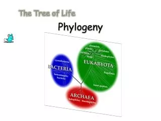
Phylogeny Ch. 7 & 8
Overview • Evolution and sequence variation • Phylogenetic trees • The meaning of distance • Evolutionary sequence models • Constructing trees • Sequence alignment
Sequence similarity may imply common descent • Similarity of genomic and protein sequence is one way to try and infer the relationships among organisms. • If two sequences are homologs, they are descended from a most recent common ancestor sequence. • This may imply that the ancestral sequence was in the ancestral organism, but horizontal transfer can occur.
Trees are a convenient way to summarize the relationships among a set of (orthologous) sequences or a set of species.
Rooted and Unrooted Trees • “Leaves” are extant species • Internal nodes are ancestral species • Adding a root gives time a direction • It is very difficult to accurately determine where the root should go, so it is best to avoid placing it…
The Data • Phylogenetic trees predate genomic sequence data. • Traditional taxonomy used physical characteristics. • Qualitative: eg, fur-bearing • Quantitative: number of petals • Sequence data is quantitative and plentiful.
What’s in a tree? • Cladograms • Additive trees • Ultrametric trees
Cladograms • Branch lengths are meaningless. • Shows evolutionary relationships of “taxa” only.
Additive Trees • Branch lengths measure “evolutionary distance”. • Total distance between two taxa is the sum of the branch lengths separating them. • Don’t have to be rooted.
But how can two species be at different “evolutionary distances” from their ancestor? ?
Distance Time • The rate of evolution, r, can vary over time. • The distance is equal to the rate times the time: d=rt
Ultrametric Trees • Simplest type of rooted, additive tree. • Assumes that the rate of evolution is constant over time. • With sequences, called the “molecular clock”. • Horizontal lines have no meaning.
We want to build phylogenetic trees from orthologous genes or proteins. • Evolutionary sequence models give us a way to model how one ancestral sequence evolves (independently) into two daughter sequences.
What is the evolutionary distance between two DNA sequences? • Align the two DNA sequences. • Count the number of places where they differ (ignoring gaps) p = D/L • Dis the number of differences and • L is the total number of aligned positions
Is p the evolutionary distance? • NO! • p is just the observed number of differences. • What is value will p tend towards as evolutionary distance increases???
All things being equal… • If all mutations (from one nucleic acid to another) are equally likely, p 3/4 • Do you see why?
So what is going on here, really? • A position can mutate to any of the 3 other nucleic acids. • If the ancestral sequence is distant, this can happen multiple times. • But all we get to see is the final result! • So a position with a different nucleic acid may be the result of one or more mutation events. • And positions with the same nucleic acid can also have had an even number of mutations. Seq 1: A ->T Seq 2: A -> T
If we model mutations as a Poisson process • Probability of no mutation in time t is exp(-rt) • Both sequences evolving so exp(-2rt) • Let d=2rt • Then 1-p = exp(-d) • So d = -ln(1-p)
Summary • So the branch lengths of the tree are “d=rt”. • We must propose an evolutionary model to compute “d” from the observed p-distance. • The Poisson model is too simple. • It doesn’t capture real evolution.
Other Evolutionary Models • Jukes-Cantor • Assumes all base frequencies are ¼ • Has one parameter, α, the substitution rate (per unit time). • Distance formula: d = ¾ ln(1- 4⁄3p)
Kimura Two-Parameter Model • Models transversions and transitions separately because the former are very uncommon in reality. • Transitions: A<->G, C<->T • Two parameters: transition rate α, transversion rate β. • Distance formula: d = ½ ln(1-2P-Q) - ¼ ln(1-2Q) where P and Q are fraction of transitions and transversions, respectively.
More General Models • More general models take into account other realities like: • Non-uniform base frequencies • Non-uniform mutation rates (Gamma correction)
First, construct a multiple alignment • A good multiple alignment is key. • The p-distances between pairs of sequences can then be computed. • This allows the d-distances between pairs of sequences to be computed. • Some tree-building methods use the multiple alignment directly • Parsimony Methods
Next, choose a tree-building method • UPGMA (1958) • Builds rooted, ultrametric trees • Assumes constant rate of evolution in all branches • Neighbor-joining (1987) • Builds unrooted, additive trees • Assumes the best tree has the shortest total branch length. • Principal of minimum evolution, as with maximum parsimony trees.
Neighbor-Joining • Similar to maximum parsimony, but works with large datasets. • Maximum parsimony methods consider many more tree topologies, so they don’t scale to large numbers of species.
Neighbors are separated by one node. • Start with a star topology. • Everybody’s a neighbor!
Neighbors are separated by one node. • Assume Sequences 1 and 2 were nearest neighbors. • So they are joined with new node Y. • The method computes the new branch lengths.
Find pair of neighbors that reduces total branch length most • N sequences • dij = distance between sequences i and j • Ui = sum of distances from sequence i to all other sequences • δij = dij - (Ui + Uj)/(N-2) Find pair of sequences with minimum δij.
Initial tree: 5 sequences A B C E D
How the new branch lengths are computed • The new branch lengths from the joined neighbors to the new node W are biW = ½(dij+ (Ui – Uj)/(N-2)) and bjW = dij – biW where i = E and j = D in the example.
Replace joined neighbors with new node W. A B A B C C E W D
Compute distances from new node W to each remaining sequence • The new distances (to each remaining sequence k) dWk = ½(dik + djk – dij) where i and j are the nearest neighbors (D and E in this example).
Replace neighbors with new node X. A A B B C X W
All done. • The tree is now a binary tree so the procedure is complete.