Phylogeny
Phylogeny. - A brief introduction in 4 hours -. Outline. Introduction Practical approach Evolutionary models Distance-based methods / TP5_1 Databases and software Sequence-based methods / TP5_2. What is p hylogeny?. P hylogeny is the evolutionary history and relationship of species. .

Phylogeny
E N D
Presentation Transcript
Phylogeny - A brief introduction in 4 hours -
Outline • Introduction • Practical approach • Evolutionary models • Distance-based methods / TP5_1 • Databases and software • Sequence-based methods / TP5_2
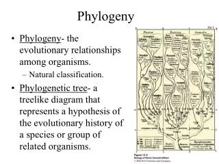
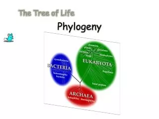
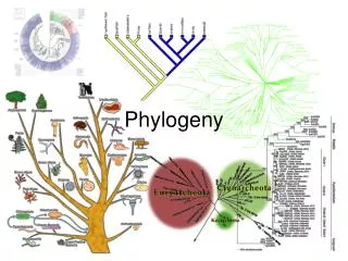
Phylogeny is the evolutionary history and relationship of species.
What data types can be used to infer phylogenies? • Morphological characters • Physiological characters • Gene order (e.g. in mitochondria) • Sequence data • Nucleotide sequences • Amino acid sequences • Mixed characters • ….
What is a phylogenetic tree? • A phylogenetic tree is a model about the evolutionary relationship between species (OTUs) based on homologous characters • But not all trees are phylogenetic trees • Dendrogram = general term for a branching diagram • Cladogram: branching diagram without branch length estimates • Phylogenetic tree or Phylogram: branching diagram with branch length estimates
What is a phylogenetic tree? • Rooted or unrooted • bifurcating or multifurcating (solved or unsolved)
Gene duplication • Prokaryots: at least 50% • Eukaryots: >90%
After gene duplication • Coexistence (normally only for a short while) • Mostly, only one copy is retained • becomes nonfunctional (non-functionalization), • becomes a pseudogene (pseudogenization) • is lost • Both copies are retained • Distinct expression pattern • Distinct subcellular location (rare) • One copy keeps the original function, the other copy acquires a new function (neofunctionalization) • Deleterious mutations in both entries (subfunctionalization)
Relationships within homologs Frog gene A Orthologs Human gene A Mouse gene A Gene duplication Paralogs Mouse gene B Homologs Ancestral gene Human gene B Orthologs Frog gene B Drosophila gene AB
Homologs … Homologs = Genes of common origin Orthologs = 1. Genes resulting from a speciation event, 2. Genes originating from an ancestral gene in the last common ancestor of the compared genomes Co-orthologs = Orthologs that have undergone lineage-specific gene duplications subsequent to a particular speciation event Paralogs = Genes resulting from gene duplication Inparalogs = Paralogs resulting from lineage-specific duplication(s) subsequent to a particular speciation event Outparalogs = Paralogs resulting from gene duplication(s) preceding a particular speciation event One-to-one (1:1) orthologs = Orthologs with no (known) lineage-specific gene duplications subsequent to a particular speciation event One-to-many (1:n) orthologs: Orthologs of which at least one - and at most all but one - has undergone lineage-specific gene duplication subsequent to a particular speciation event Many-to-many (n:n) orthologs = Orthologs which have undergone lineage-specific gene duplications subsequent to a particular speciation event Xenologs = Orthologs derived by horizontal gene transfer from another lineage
Relationships between orthologs and paralogs Frog gene A Orthologs (Group 1) Human gene A Mouse gene A Co-orthologs of Drosophila gene AB Gene duplication Inparalogs of Group 2 Orthologs (Group 2) Mouse gene B Ancestral gene Human gene B Outparalogs of Group 1 Frog gene B Drosophila gene AB
Practical approach I Actin-related protein 2 (first 60 columns of the alignment) ARP2_A MESAP---IVLDNGTGFVKVGYAKDNFPRFQFPSIVGRPILRAEEKTGNVQIKDVMVGDE ARP2_B MDSQGRKVIVVDNGTGFVKCGYAGTNFPAHIFPSMVGRPIVRSTQRVGNIEIKDLMVGEE ARP2_C MDSQGRKVVVCDNGTGFVKCGYAGSNFPEHIFPALVGRPIIRSTTKVGNIEIKDLMVGDE ARP2_D MDSQGRKVVVCDNGTGFVKCGYAGSNFPEHIFPALVGRPIIRSTTKVGNIEIKDLMVGDE ARP2_E MDSKGRNVIVCDNGTGFVKCGYAGSNFPTHIFPSMVGRPMIRAVNKIGDIEVKDLMVGDE *:* :* ******** *** *** . **::****::*: . *::::**:***:* Species are: Caenorhabditis briggsae Drosophila melanogaster Homo sapiens Mus musculus Schizosaccharomyces pombe Can you build a dendrogram (tree) for the sequences of the alignment? Can you assign the species to the corresponding sequences of the alignment?
Phylogenetic analysis • Select Data • Alignment • Select a data model • Select a substitution model • Tree-building • [Distance matrix] • Tree-building • Tree evaluation
Select data • To be considered: • Input data must be homolog! • Number of character states • Content of phylogenetic information • Size of the dataset • Automated cluster data from large datasets • etc
Alignment • MSA methods • ClustalW • muscle • MAFFT • Probcons • T-coffee • … • See previous course …
Data model = Characters selected for the analysis • To be considered: • Each character should be homolog! • Missing data (in some OTU) • Number of characters • etc
Evolutionary models Phylogenetic tree-building presumes particular evolutionary models The model used influences the outcome of the analysis and should be considered in the interpretation of the analysis results • Which aspects are to be considered? • Frequencies of aa exchange • Change of aa frequencies during evolution • Between-site rate variation or Among-site substitution rate heterogenity • Presence of invariable sites
Evolutionary models Notation, e.g. JTT JTT + F JTT + F + gamma (4 ) JTT + F + gamma (8 ) + I (under discussion) JTT + F + I It is not always the most complex model that produces the best result. The more complex the model, the more complex the explanation of the results.
Tree-building methods • Distance (matrix) methods • Calculate distances for all pairs of taxa based on the sequence alignment • Construct a phylogenetic tree based on a distance matrix • Character-based (Sequence) methods • Constructs a phylogenetic tree based on the sequence alignment
Step 1: Compute distances • Estimate the number of amino acid substitutions between sequence pairs p distance: p=nd/n p = proportion (p distance) nd= number of aa differences n = number of aa used ^
Step 1: Compute distances • Nonlinear relationship of p with t (time) • Estimation of aa substitutions • Poisson correction • PC distance • Gamma correction • Gamma distance
Step 2: Tree-building Common distance methods • Neighbor Joining (NJ) • UPGMA / WPGMA • Least Square (LS) • Minimal Evolution (ME)
Neighbor Joining (NJ) • Saitou, Nei (1987) • Principle • Clustering method • Simplified minimal evolution principle • Neighbors = taxa connected by a single node in an unrooted tree • Computational process: Star tree, followed by a successive joining of neighbors and the creation of new pairs of neighbors • Result: • A single final tree with branch length estimates • unrooted tree
Neighbor Joining (NJ) • Sum of branch lengths in the star tree • Calculate the sum of all branch lengths for all possible neighbors …
Neighbor Joining (NJ) • Calculate Length X-Y • Calculate again sum of all branch length
Neighbor Joining (NJ) • Advantage • Very efficient • Also for large datasets • Disadvantage • Does not examine all possible topologies
Bootstrap • Used to test the robustness of a tree topology • by Bradley Efron (1979) • Felsenstein (1985) • Principle: new MSA datasets are created by choosing randomly N columns from the original MSA; where N is the length of the original MSA • 100-1000 replicates • Bootstrap support values: (75%), 95%, 98%
TP5 - 1st part, Exercises 1-5 http://education.expasy.org/m07_phylo.html
Ortholog databases & phylogenetic databases Some databases providing orthologous groups and trees • COG/KOG • HOGENOM • Ensembl • OMA browser • OrthoDB • OrthoMCL • Pfam • PANDIT • SYSTERS • TreeBase • Tree of Life
Phylogenetic software Software packages • Freely available • Phylip • BioNJ • PhyML • Tree Puzzle • MrBayes • Commercial • PAUP • MEGA
Phylogenetic servers • http://www.phylogeny.fr/ • http://bioweb.pasteur.fr/seqanal/phylogeny/intro-uk.html • http://atgc.lirmm.fr/phyml/ • http://phylobench.vital-it.ch/raxml-bb/ • http://www.fbsc.ncifcrf.gov/app/htdocs/appdb/drawpage.php?appname=PAUP • http://power.nhri.org.tw/power/home.htm
Sequence methods Most common: • Maximum Parsimony (MP) • Maximum Likelihood (ML) • Baysian Inference
Maximum Parsimony (MP) • Originally developed for morphological characters • Henning, 1966 • William of Ockham: the best hypothesis is the one that requires the smallest number of assumptions
Maximum Parsimony (MP) • Principle: • Estimate the minimum number of substitutions for a given topology • Parsimony-informative sites (exclude invariable sites and singletons) • Searching MP trees • Exhaustive search • Branch-and-bound (Hendy-Penny, 1982) • Good but time-consuming, if m>20 • Heuristic search • Result tree might not be the most parsimonious tree • Result • Multiple result trees are possible (strict consensus tree, majority-rule consensus tree) • Most parsimonious tree vs true tree • Unrooted result trees
Maximum Parsimony (MP) • Advantages • Free from assumptions (model-free) • Disadvantages • Does not take into account homoplasy • Long-branch attraction (LBA): creates wrong topologies, if the substitution rate varies extensively between lineages
Maximum Likelihood (ML) • Cavalli-Sforza, Edwards (1967), gene frequency data • Felsenstein (1981), nucleotide sequences • Kishino (1990), proteins • Principle • Maximizes the likelihood of observing the sequence data for a specific model of character state changes • Likelihood of a site = Sum of probabilities of every possible reconstruction of ancestral states at the internal nodes • Likelyhood of the tree = Product of the likelihoods for all sites (=sum of log likelihoods) • Result = tree with the highest likelihood • Maximized to estimate branch lengths, not topologies • Search strategies: rarely exhaustive, mostly heuristic • NNI (Nearest neighbor interchanges) • TBR (Tree bisection-reconnection) • SPR (Subtree pruning and regrafting)
Number of possible trees • Unrooted bifurcating trees: • Rooted bifurcating trees:
Number of possible trees Rooted Unrooted Leaves
Number of possible trees Leaves Unrooted Rooted 3 1 3 4 3 15 5 15 105 6 105 945 7 945 10395 8 10395 135135 9 135135 2027025 10 2027025 34459425
Maximum Likelihood (ML) • Methods: • ProML (Phylip) • PhyML • RaxML • …
Tree evaluation • Topology • Comparison with species tree • Robustness, e.g. bootstrap • Branch lengths
TP5 – 2nd part, Exercise 6 http://education.expasy.org/m07_phylo.html