DNA Sequencing
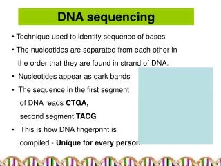
DNA Sequencing. cut many times at random. Whole Genome Shotgun Sequencing. genome. plasmids (2 – 10 Kbp). forward-reverse paired reads. known dist. cosmids (40 Kbp). ~500 bp. ~500 bp. Steps to Assemble a Genome. Some Terminology read a 500-900 long word that comes


DNA Sequencing
E N D
Presentation Transcript
cut many times at random Whole Genome Shotgun Sequencing genome plasmids (2 – 10 Kbp) forward-reverse paired reads known dist cosmids (40 Kbp) ~500 bp ~500 bp
Steps to Assemble a Genome Some Terminology read a 500-900 long word that comes out of sequencer mate pair a pair of reads from two ends of the same insert fragment contig a contiguous sequence formed by several overlapping reads with no gaps supercontig an ordered and oriented set (scaffold) of contigs, usually by mate pairs consensus sequence derived from the sequene multiple alignment of reads in a contig 1. Find overlapping reads 2. Merge some “good” pairs of reads into longer contigs 3. Link contigs to form supercontigs 4. Derive consensus sequence ..ACGATTACAATAGGTT..
2. Merge Reads into Contigs • Overlap graph: • Nodes: reads r1…..rn • Edges: overlaps (ri, rj, shift, orientation, score) Reads that come from two regions of the genome (blue and red) that contain the same repeat Note: of course, we don’t know the “color” of these nodes
repeat region 2. Merge Reads into Contigs We want to merge reads up to potential repeat boundaries Unique Contig Overcollapsed Contig
repeat region 2. Merge Reads into Contigs • Ignore non-maximal reads • Merge only maximal reads into contigs
2. Merge Reads into Contigs • Remove transitively inferable overlaps • If read r overlaps to the right reads r1, r2, and r1 overlaps r2, then (r, r2) can be inferred by (r, r1) and (r1, r2) r r1 r2 r3
Overlap graph after forming contigs Unitigs: Gene Myers, 95
Repeats, errors, and contig lengths • Repeats shorter than read length are easily resolved • Read that spans across a repeat disambiguates order of flanking regions • Repeats with more base pair diffs than sequencing error rate are OK • We throw overlaps between two reads in different copies of the repeat • To make the genome appear less repetitive, try to: • Increase read length • Decrease sequencing error rate Role of error correction: Discards up to 98% of single-letter sequencing errors decreases error rate decreases effective repeat content increases contig length
3. Link Contigs into Supercontigs Normal density Too dense Overcollapsed Inconsistent links Overcollapsed?
3. Link Contigs into Supercontigs Find all links between unique contigs Connect contigs incrementally, if 2 links supercontig (aka scaffold)
3. Link Contigs into Supercontigs Fill gaps in supercontigs with paths of repeat contigs
4. Derive Consensus Sequence TAGATTACACAGATTACTGA TTGATGGCGTAA CTA Derive multiple alignment from pairwise read alignments TAGATTACACAGATTACTGACTTGATGGCGTAAACTA TAG TTACACAGATTATTGACTTCATGGCGTAA CTA TAGATTACACAGATTACTGACTTGATGGCGTAA CTA TAGATTACACAGATTACTGACTTGATGGGGTAA CTA TAGATTACACAGATTACTGACTTGATGGCGTAA CTA Derive each consensus base by weighted voting (Alternative: take maximum-quality letter)
Some Assemblers • PHRAP • Early assembler, widely used, good model of read errors • Overlap O(n2) layout (no mate pairs) consensus • Celera • First assembler to handle large genomes (fly, human, mouse) • Overlap layout consensus • Arachne • Public assembler (mouse, several fungi) • Overlap layout consensus • Phusion • Overlap clustering PHRAP assemblage consensus • Euler • Indexing Euler graph layout by picking paths consensus
Quality of assemblies—mouse Terminology:N50 contig length If we sort contigs from largest to smallest, and start Covering the genome in that order, N50 is the length Of the contig that just covers the 50th percentile. 7.7X sequence coverage
Quality of assemblies—dog 7.5X sequence coverage
History of WGA 1997 • 1982: -virus, 48,502 bp • 1995: h-influenzae, 1 Mbp • 2000: fly, 100 Mbp • 2001 – present • human (3Gbp), mouse (2.5Gbp), rat*, chicken, dog, chimpanzee, several fungal genomes Let’s sequence the human genome with the shotgun strategy That is impossible, and a bad idea anyway Phil Green Gene Myers
Genomes Sequenced • http://www.genome.gov/10002154
1 4 3 5 2 5 2 3 1 4 Phylogeny Tree Reconstruction
Phylogenetic Trees • Nodes: species • Edges: time of independent evolution • Edge length represents evolution time • AKA genetic distance • Not necessarily chronological time
Inferring Phylogenetic Trees Trees can be inferred by several criteria: • Morphology of the organisms • Can lead to mistakes! • Sequence comparison Example: Orc: ACAGTGACGCCCCAAACGT Elf: ACAGTGACGCTACAAACGT Dwarf: CCTGTGACGTAACAAACGA Hobbit: CCTGTGACGTAGCAAACGA Human: CCTGTGACGTAGCAAACGA
Phylogeny and sequence comparison Basic principles: • Degree of sequence difference is proportional to length of independent sequence evolution • Only use positions where alignment is certain – avoid areas with (too many) gaps
Distance between two sequences Given sequences xi, xj, Define dij = distance between the two sequences One possible definition: dij = fraction f of sites u where xi[u] xj[u] Better scores are derived by modeling evolution as a continuous change process – not covered here Jukes Kantor, Kimura, etc.
A simple clustering method for building tree UPGMA (unweighted pair group method using arithmetic averages) Or the Average Linkage Method Given two disjoint clusters Ci, Cj of sequences, 1 dij = ––––––––– {p Ci, q Cj}dpq |Ci| |Cj| Claim that if Ck = Ci Cj, then distance to another cluster Cl is: dil |Ci| + djl |Cj| dkl = –––––––––––––– |Ci| + |Cj| Proof Ci,Cl dpq + Cj,Cl dpq dkl = –––––––––––––––– (|Ci| + |Cj|) |Cl| |Ci|/(|Ci||Cl|) Ci,Cl dpq + |Cj|/(|Cj||Cl|) Cj,Cl dpq = –––––––––––––––––––––––––––––––––––– (|Ci| + |Cj|) |Ci| dil + |Cj| djl = ––––––––––––– (|Ci| + |Cj|)
Algorithm: Average Linkage 1 4 Initialization: Assign each xi into its own cluster Ci Define one leaf per sequence, height 0 Iteration: Find two clusters Ci, Cj s.t. dij is min Let Ck = Ci Cj Define node connecting Ci, Cj, & place it at height dij/2 Delete Ci, Cj Termination: When two clusters i, j remain, place root at height dij/2 3 5 2 5 2 3 1 4
Example 4 3 2 1 v w x y z
Ultrametric Distances and Molecular Clock Definition: A distance function d(.,.) is ultrametric if for any three distances dij dik dij, it is true that dij dik = dij The Molecular Clock: The evolutionary distance between species x and y is 2 the Earth time to reach the nearest common ancestor That is, the molecular clock has constant rate in all species The molecular clock results in ultrametric distances years 1 4 2 3 5
Ultrametric Distances & Average Linkage Average Linkage is guaranteed to reconstruct correctly a binary tree with ultrametric distances Proof: Exercise 5 1 4 2 3
Weakness of Average Linkage Molecular clock: all species evolve at the same rate (Earth time) However, certain species (e.g., mouse, rat) evolve much faster Example where UPGMA messes up: AL tree Correct tree 3 2 1 3 4 4 2 1
d1,4 Additive Distances 1 Given a tree, a distance measure is additive if the distance between any pair of leaves is the sum of lengths of edges connecting them Given a tree T & additive distances dij, can uniquely reconstruct edge lengths: • Find two neighboring leaves i, j, with common parent k • Place parent node k at distance dkm = ½ (dim + djm – dij) from any node m i, j 4 12 8 3 13 7 9 5 11 10 6 2
Reconstructing Additive Distances Given T x T D y 5 4 3 z 3 4 w 7 6 v If we know T and D, but do not know the length of each leaf, we can reconstruct those lengths
Reconstructing Additive Distances Given T x T D y z w v
Reconstructing Additive Distances Given T D x T y z a w D1 v dax = ½ (dvx + dwx – dvw) day = ½ (dvy + dwy – dvw) daz = ½ (dvz + dwz – dvw)
Reconstructing Additive Distances Given T D1 x T y 5 4 b 3 z 3 a 4 c w 7 D2 6 d(a, c) = 3 d(b, c) = d(a, b) – d(a, c) = 3 d(c, z) = d(a, z) – d(a, c) = 7 d(b, x) = d(a, x) – d(a, b) = 5 d(b, y) = d(a, y) – d(a, b) = 4 d(a, w) = d(z, w) – d(a, z) = 4 d(a, v) = d(z, v) – d(a, z) = 6 Correct!!! v D3
Neighbor-Joining • Guaranteed to produce the correct tree if distance is additive • May produce a good tree even when distance is not additive Step 1: Finding neighboring leaves Define Dij = (N – 2) dij – kidik – kjdjk Claim: The above “magic trick” ensures that Dij is minimal iffi, j are neighbors 1 3 0.1 0.1 0.1 0.4 0.4 4 2
Algorithm: Neighbor-joining Initialization: Define T to be the set of leaf nodes, one per sequence Let L = T Iteration: Pick i, j s.t. Dij is minimal Define a new node k, and set dkm = ½ (dim + djm – dij) for all m L Add k to T, with edges of lengths dik = ½ (dij + ri – rj), djk = dij – dik where ri = (N – 2)-1kidik Remove i, j from L; Add k to L Termination: When L consists of two nodes, i, j, and the edge between them of length dij
Parsimony – direct method not using distances • One of the most popular methods: • GIVEN multiple alignment • FIND tree & history of substitutions explaining alignment Idea: Find the tree that explains the observed sequences with a minimal number of substitutions Two computational subproblems: • Find the parsimony cost of a given tree (easy) • Search through all tree topologies (hard)
Example: Parsimony cost of one column {A} Final cost C = 1 {A} {A, B} Cost C+=1 A B A A A A B A {B} {A} {A} {A}
Parsimony Scoring Given a tree, and an alignment column u Label internal nodes to minimize the number of required substitutions Initialization: Set cost C = 0; node k = 2N – 1 (last leaf) Iteration: If k is a leaf, set Rk = { xk[u] } // Rk is simply the character of kth species If k is not a leaf, Let i, j be the daughter nodes; Set Rk = Ri Rj if intersection is nonempty Set Rk = Ri Rj, and C += 1, if intersection is empty Termination: Minimal cost of tree for column u, = C
Example {B} {A,B} {A} {B} {A} {A,B} {A} A A A A B B A B {A} {A} {A} {A} {B} {B} {A} {B}
Traceback to find ancestral nucleotides Traceback: • Choose an arbitrary nucleotide from R2N – 1 for the root • Having chosen nucleotide r for parent k, If r Ri choose r for daughter i Else, choose arbitrary nucleotide from Ri Easy to see that this traceback produces some assignment of cost C
Example Admissible with Traceback x B Still optimal, but inadmissible with Traceback A {A, B} B A x {A} B A A B B {A, B} x B x A A B B A A A B B {B} {A} {A} {B} A x A x A A B B
Probabilistic Methods A more refined measure of evolution along a tree than parsimony P(x1, x2, xroot | t1, t2) = P(xroot) P(x1 | t1, xroot) P(x2 | t2, xroot) If we use Jukes-Cantor, for example, and x1 = xroot = A, x2 = C, t1 = t2 = 1, = pA¼(1 + 3e-4α) ¼(1 – e-4α) = (¼)3(1 + 3e-4α)(1 – e-4α) xroot t1 t2 x1 x2
Probabilistic Methods xroot • If we know all internal labels xu, P(x1, x2, …, xN, xN+1, …, x2N-1 | T, t) = P(xroot)jrootP(xj | xparent(j), tj, parent(j)) • Usually we don’t know the internal labels, therefore P(x1, x2, …, xN | T, t) = xN+1 xN+2 … x2N-1P(x1, x2, …, x2N-1 | T, t) xu x2 xN x1
Felsenstein’s Likelihood Algorithm Let P(Lk | a) denote the prob. of all the leaves below node k, given that the residue at k is a To calculate P(x1, x2, …, xN | T, t) Initialization: Set k = 2N – 1 Iteration: Compute P(Lk | a) for all a If k is a leaf node: Set P(Lk | a) = 1(a = xk) If k is not a leaf node: 1. Compute P(Li | b), P(Lj | b) for all b, for daughter nodes i, j 2. Set P(Lk | a) = b,c P(b | a, ti) P(Li | b) P(c | a, tj) P(Lj | c) Termination: Likelihood at this column = P(x1, x2, …, xN | T, t) = aP(L2N-1 | a)P(a)
Probabilistic Methods Given M (ungapped) alignment columns of N sequences, • Define likelihood of a tree: L(T, t) = P(Data | T, t) = m=1…M P(x1m, …, xnm, T, t) Maximum Likelihood Reconstruction: • Given data X = (xij), find a topology T and length vector t that maximize likelihood L(T, t)
Current popular methods HUNDREDS of programs available! http://evolution.genetics.washington.edu/phylip/software.html#methods Some recommended programs: • Discrete—Parsimony-based • Rec-1-DCM3 http://www.cs.utexas.edu/users/tandy/mp.html Tandy Warnow and colleagues • Probabilistic • SEMPHY http://www.cs.huji.ac.il/labs/compbio/semphy/ Nir Friedman and colleagues