Download
1 / 22
220 likes | 343 Vues
The IceCube Neutrino Observatory, located at the South Pole, is a groundbreaking facility designed to detect neutrinos over a wide energy range, from 10^7 eV to 10^20 eV. Comprised of 80 strings of optical sensors, it spans an instrumental volume of 1 km³, allowing for the detection of neutrinos from various astrophysical sources such as gamma-ray bursts (GRBs) and active galactic nuclei (AGNs). This observatory plays a crucial role in advancing our understanding of high-energy cosmic phenomena and enhances our capability to study stable particles like muons, photons, and neutrinos.

E N D
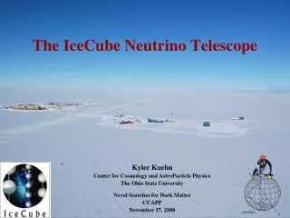
A km3 Neutrino Telescope: IceCube at the South Pole Howard Matis - LBNL for the IceCube Collaboration
Neutrino Astronomymeasuring ns by its µ Accelerator Target • Stable particles: p, • Astrophysical Sources • GRB, AGN, Super Novae • GZK (p +CMB ) • Topological defects • Backgrounds • Atmospheric ’s • Atmospheric ’s Earth IceCube H. Matis – Lawrence Berkeley National Laboratory
IceTop South Pole Skiway 1400 m 2400 m IceCube • IceCube is designed to detect neutrinos of all flavors at energies from 107 eV (SN) to 1020 eV • 80 Strings • 4800 PMT • Instrumented volume: 1 km3 • Depth: 1400 m to 2400m Amanda H. Matis – Lawrence Berkeley National Laboratory
South Pole Dark sector Skiway AMANDA Dome IceCube H. Matis – Lawrence Berkeley National Laboratory
Detecting ns • ns interact in earth • Produce µ (follows path of n) • Detect Cherenkov light in ice with phototubes buried in the ice • Detect upward µs • Ice filters downward cosmic µs H. Matis – Lawrence Berkeley National Laboratory
Simulated nm + N m- + X 1 Km Eµ=10 TeV Eµ= 6 PeV • Measure m energy at the detector by counting the number of fired PMTs and the total light. H. Matis – Lawrence Berkeley National Laboratory
Other Reactions ne + N e- + X nt + N t- + X nt t PeVt(300 m) t decays • Electron Cascade • 1 PeV ≈ 500 m diameter H. Matis – Lawrence Berkeley National Laboratory
IceCubeString 60 optical sensors/string OM Spacing: 17 m Main Cable DOM HV and Base 1400 m String Gel photomultiplier Glass pressure sphere rated to 10,000 psi Outer diameter: 13” 2400 m H. Matis – Lawrence Berkeley National Laboratory
Self-triggers on each pulse Captures waveforms Time-stamps each pulse Digitizes waveforms Performs feature extraction Buffers data Responds to Surface DAQ Set PMT HV, threshold, etc Digital Optical Module - (DOM) DOM Board 33 cm H. Matis – Lawrence Berkeley National Laboratory
Requirements for One ElementDigital Optical Module (DOM) • Time resolution: < 5 ns rms • Waveform capture • > 250 MHzfor first 500 ns • ~ 40 MHzfor 5000 ns • Dynamic Range • > 200 PE / 15 ns • > 2000 PE / 5000 ns • Dead-time < 1% • OM noise rate < 500 Hz(40K in glass sphere) • 1 to 10,000 photons that are incident over several µs High dynamic range waveform recording H. Matis – Lawrence Berkeley National Laboratory
Time Synch-ronizing Modules Surface DOM dt Dtdown =Dtup=1/2(Tround-trip- dt) H. Matis – Lawrence Berkeley National Laboratory
DAQ Network Architecture String - Electronics in the ice Global Timing H. Matis – Lawrence Berkeley National Laboratory
AMANDA String 18 • Springboard for transition to IceCube • 41 DOMs deployed in 99/00 season; 37 operational • Test bed: download new code into ice • Communicate and program in North America H. Matis – Lawrence Berkeley National Laboratory
String 18 DOM Board Oscillator H. Matis – Lawrence Berkeley National Laboratory
Digital ATWD Waveforms Hi Gain Single Photon ADC Spectra “Bucket” Low Gain “Bucket” No Gain ADC Charge “Bucket” Complex Waveform @600 MHz Clock Digitalization @ ~ 600 Hz “Bucket” “Slow” ADC “Bucket” • ATWD Channels 1 - 4: 1.7 ns/sample for 217 ns • ADC: 60 ns/sample for 7.7 ms Time H. Matis – Lawrence Berkeley National Laboratory
Timing with “Phone Wire” to few ns • Transit time for 2.5 km twisted pair: ~12 s • Rise-time after propagation ~ 2 s (~1/t) • Use a bipolar “Time-Mark” signal pulse • Digitize time-mark pulse @ 20 MHz, 10-bit • Fit leading edge & baseline : 3.5 ns rms H. Matis – Lawrence Berkeley National Laboratory
Timing with µs T (DOMN) 12 m Dt - ns T (DOMN+1) • DT = T (DOMN) - T (DOMN+1) • Two clear components: • random coincidences (flat) • correlated light (peak at ~ 0) H. Matis – Lawrence Berkeley National Laboratory
Reconstructed m Event • Only first hit in each OM shown • Down flow of light • No “early photons” • Late hits consistent with: • light scattering, or • a second m? • Down going m H. Matis – Lawrence Berkeley National Laboratory
String 18 Performance • Timing: 3.5 ns rms(very stable) • SPE spectrum: as expected • PMT Gain Drift: <<0.2 %/week • LED Beacons: ~8 ns rms(ice optics) • Down going : observed • µ waveforms: ~15% have > 1 “hit” H. Matis – Lawrence Berkeley National Laboratory
Summary • IceCube – New detector under development to explore astrophysical ns • Decentralized timing with digital technology • Measure full waveform • Provides more information for reconstruction • More detail for physics discovery • Feature extraction - less data to record and transmit • Can synchronize separate and remote elements to several ns • Fully functional prototypes tested with muons in AMANDA • Prototypes meet or exceed IceCube requirements H. Matis – Lawrence Berkeley National Laboratory
IceCube Collaboration Institutions: 11 US, 9 European, 1 Japanese and 1 Venezuelan; Bartol Research Institute, University of Delaware (*) BUGH Wuppertal, Germany (*) Universite Libre de Bruxelles, Brussels, Belgium (*) CTSPS, Clark-Atlanta University, Atlanta, USA DESY-Zeuthen, Zeuthen, Germany (*) Institute for Advanced Study, Princeton, USA Lawrence Berkeley National Laboratory, Berkeley, USA(*) Department of Physics, Southern University and A\&M College, Baton Rouge, LA, USA Dept. of Physics, UC Berkeley, USA (*) Institute of Physics, University of Mainz, Mainz, Germany(*) University of Mons-Hainaut, Mons, Belgium (*) Dept. of Physics and Astronomy, University of Pennsylvania, Philadelphia, USA (*) Dept. of Astronomy, Dept. of Physics, SSEC, University of Wisconsin, Madison, USA (*) Physics Department, University of Wisconsin, River Falls, USA (*) Division of High Energy Physics, Uppsala University, Uppsala, Sweden (*) Dept. of Physics, Stockholm University, Stockholm, Sweden (*) Dept. of Physics, University of Alabama, USA Vrije Universiteit Brussel, Brussel, Belgium (*) Chiba University, Japan Dept. of Astrophysics, Imperial College, UK Dept. of Physics, University of Maryland, USA Universidad Simon Bolivar, Caracas, Venezuela (*) also in AMANDA H. Matis – Lawrence Berkeley National Laboratory
The End H. Matis – Lawrence Berkeley National Laboratory