Performance Bounds in Pattern Recognition: ROC Curves and Classifier Comparisons
This lecture delves into performance bounds in pattern recognition, focusing on ROC curves, Chernoff bound, and Bhattacharyya bound which provide insights into classifier performance. We examine the dichotomizer's decision-making process and thresholds, especially in Gaussian classifiers. Understanding these bounds is vital for deriving closed-form solutions to complex problems. The ROC curve is particularly useful for comparing different classification systems under varying conditions, ensuring effective decision-making through visual analysis of true positive and false positive rates.

Performance Bounds in Pattern Recognition: ROC Curves and Classifier Comparisons
E N D
Presentation Transcript
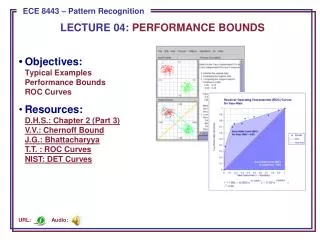
ECE 8443 – Pattern Recognition LECTURE 04: PERFORMANCE BOUNDS • Objectives:Typical ExamplesPerformance BoundsROC Curves • Resources:D.H.S.: Chapter 2 (Part 3)V.V.: Chernoff BoundJ.G.: BhattacharyyaT.T. : ROC CurvesNIST: DET Curves Audio: URL:
Two-Category Case (Review) • A classifier that places a pattern in one of two classes is often referred to as a dichotomizer. • We can reshape the decision rule: • If we use log of the posterior probabilities: • A dichotomizer can be viewed as a machine that computes a single discriminant function and classifies x according to the sign (e.g., support vector machines).
Threshold Decoding (Review) • This has a simple geometric interpretation: • The decision region when the priors are equal and the support regions are spherical is simply halfway between the means (Euclidean distance).
Identity Covariance • Case: i= 2I • This can be rewritten as:
Equal Covariances • Case: i=
Error Bounds • Bayes decision rule guarantees lowest average error rate • Closed-form solution for two-class Gaussian distributions • Full calculation for high dimensional space difficult • Bounds provide a way to get insight into a problem andengineer better solutions. • Need the following inequality: • Assume a b without loss of generality: min[a,b] = b. • Also, ab(1- ) = (a/b)b and (a/b) 1. • Therefore, b (a/b)b, which implies min[a,b] ab(1- ). • Apply to our standard expression for P(error).
Chernoff Bound • Recall: • Note that this integral is over the entire feature space, not the decision regions (which makes it simpler). • If the conditional probabilities are normal, this expression can be simplified.
where: Chernoff Bound for Normal Densities • If the conditional probabilities are normal, our bound can be evaluated analytically: • Procedure: find the value of that minimizes exp(-k( ), and then compute P(error) using the bound. • Benefit: one-dimensional optimization using
where: Bhattacharyya Bound • The Chernoff bound is loose for extreme values • The Bhattacharyya bound can be derived by = 0.5: • These bounds can still be used if the distributions are not Gaussian (why? hint: Occam’s Razor). However, they might not be adequately tight.
Receiver Operating Characteristic (ROC) • How do we compare two decision rules if they require different thresholds for optimum performance? • Consider four probabilities:
One system can be considered superior to another only if its ROC curve lies above the competing system for the operating region of interest. General ROC Curves • An ROC curve is typically monotonic but not symmetric:
Summary • Gaussian Distributions: how is the shape of the decision region influenced by the mean and covariance? • Bounds on performance (i.e., Chernoff, Bhattacharyya) are useful abstractions for obtaining closed-form solutions to problems. • A Receiver Operating Characteristic (ROC) curve is a very useful way to analyze performance and select operating points for systems. • Discrete features can be handled in a way completely analogous to continuous features.