Dynamic Segment Trees and Union Copy Stuctures
650 likes | 845 Vues
Dynamic Segment Trees and Union Copy Stuctures. Computational Geometry, WS 2006/07 Lecture 19 Prof. Dr. Thomas Ottmann. Algorithmen & Datenstrukturen, Institut für Informatik Fakultät für Angewandte Wissenschaften Albert-Ludwigs-Universität Freiburg. Traditional Segment Trees.

Dynamic Segment Trees and Union Copy Stuctures
E N D
Presentation Transcript
Dynamic Segment Trees and Union Copy Stuctures Computational Geometry, WS 2006/07 Lecture 19 Prof. Dr. Thomas Ottmann Algorithmen & Datenstrukturen, Institut für Informatik Fakultät für Angewandte Wissenschaften Albert-Ludwigs-Universität Freiburg
Segment Trees - motivation When one wants to inspect a small portion of a large and complex objects.Example: • GIS: windowing query in a map - given a detailed map contains enormous amount of data, the system has to determine efficiently the part of the map corresponding to a specified region (window).
Semi dynamic segment trees • Let I = { [x1, x1’ ], [x2, x2’ ],, [xn, xn’ ] } be a set of n intervals. • Let p1, p2,, pm be the list of distinct intervals endpoints, sorted from left to right. The elementary intervals are defined to be : (-, p1), [p1, p1], (p1, p2), [p2, p2],(pm,) pm p1 p2
Constructing a segment tree • A balanced binary tree T. The leaves of T correspond to the elementary intervals (ordered from left to right). The elementary interval in a leaf is denoted Int() • The internal nodes of T correspond to the intervals that are the union of elementary intervals: Int(v) is the union of intervals of its two children.
Constructing a segment tree - cont. • Each node or leaf v in T stores the interval Int(v) and a canonical set I(v) I of intervals. This set contains the intervals [x, x’] I s.t Int(v) [x, x’] and Inv(Parent(v)) [x, x’] . • Lemma: A segment tree on a set of n intervals uses O(n log n) storage.
S2, S5 S5 S1 S3 S1 S1 S4,S3 S2, S5 S4 S3 p7 p1 p3 p4 p6 p2 p5 s3 s2 s1 s5 s4 Segment tree- example
Lemma - proof T is a balances binary tree its height is O(log n). Claim: any interval [x, x’]is stored in the set I(v) for at most two nodes at the same depth of T. Proof: Let v1, v2, v3 be three nodes from left to right in same depth. Suppose [x, x’] is at v1 and v3. [x, x’]spans the interval from left point of Int(v1) to right point of Int(v3), v2lies between v1, v3 Int(parent(v2)) [x, x’] .
v2 v1 v3 Lemma - proof. Continue Any interval is stored at most twice at a given depth of T. The total amount of storage is O(n log n).
Algorithm: Query Segment Tree(V,qx) • Input: the root of a segment tree and a query point qx. • Output: All intervals in the tree containing qx. • Report all intervals in I(v). • If v is not a leaf • then if qx Int(lc(v)) • then QuerySegmentTree(lc(v), qx) • else QuerySegmentTree(rc(v), qx)
Algorithm: Query Segment Tree(V,qx) - Complexity. • Visit O(log n) nodes in total. • At each node v spend O(1 + kv) time. The intervals containing a query point qxare reported in O(log n + k) time, where k is the number of reported intervals.
Algorithm:Constructing a segment tree. • Sort the endpoints of the intervals and get the elementary intervals. • Construct a balanced binary tree on the elementary intervals and determine Int(v) for each v. (bottom-up manner). • Determine the canonical subsets : insert the intervals one by one to T.
Algorithm:Insert Segment Tree(V,[x,x’]) • Input: the root of a segment tree and an interval. • Output: The interval will be stored in tree. If Inv(v) [ x, x’] then store [ x, x’] at v. else if Int(lc(v)) [ x, x’] then InsertSegmentTree(lc(v), [ x, x’]) if Inv(rc(v)) [ x, x’] then InsertSegmentTree(rc(v), [ x, x’])
Algorithm: Insert Segment Tree(V,[x,x’]) - Complexity. • An interval is stored at most twice at each level. • There is at most one node at every level whose interval contains x (the same for x’). • Hence, We visit at most 4 nodes per level. The insertion time is O(log n). Construction time is O(n log n).
Introduction • Generalization of union-find problem: copy operation is also supported. • The structure: A bipartite graph with two node sets V1, V2 and edges between them. • V1 form the sets and V2 form the elements. An edge between v1V1 and v2V2 indicates that v2 is a member element of the set v1.
Notations • Let = {S1, Sm} be a collection of sets. • = {x1,, xn} be a collection of elements. • The sets in are subsets of . • Let x be the collection of sets that contain an element x.
The structure Consists four ingredients: • Set nodes - . • Element nodes - . • Normal nodes - connect sets to elements. • Reversed nodes - connect elements to sets. Whenever there is a path from a set node to an element node, the corresponding element is in the corresponding set.
The structure - continue. The following invariant are maintained: • A set node has one outgoing edge. • An element node has one incoming edge. • A normal node has one incoming edge, and at least two outgoing edges. • A reversed node has one outgoing edge and at least two incoming edges. • No edge may go from a reversed node to another reversed node.
The structure - continue. • No edge may go from a normal node to another normal node. • There is one unique path from a set node to an element node iff the element is in the set. • Any path in the union-copy structure from a set node to an element node consists of an alternating sequence of normal and reversed nodes. The union copy structure is acyclic.
set S2 S3 S5 S1 S4 normal reversed element x4 x2 x7 x6 x1 x3 x5 x8 The structure - example
Defining the operations. • Set-create(S) - create a new empty set in with name S. • Set-insert(Si, xj) - (defined when xj Si). make Si Si {xj}. • Set-destroy(Si) - remove Si from . • Set-find(Si) - report all elements in Si. • Set-union(Si, Sj) - (defined when Si, Sj disjoint). Si Si Sj and Sj. • Set-copy(Si, Sj) - (defined when Sj is empty). Sj Si.
Defining the operations. Continue • Element-create(x) - create an element x in and x . • Element-insert(xi, Sj) - (define when xi Sj)xi xi {Sj}. • Element-destroy(xi) - remove xi from and from all its sets. • Element-find(xi) - report all sets that contain xi. • Element-union(xi, xj) - (defined when no set contains them both). Sxj, S S {xi}\{xj}, hence xi becomes xi xj and xj . • Element-copy(xi, xj) - (defined when xj in no set). Puts xj in all sets containing xi.
S2 S3 S5 S1 S4 x4 x2 x7 x6 x1 x3 x5 x8 Set-insert(S4,x2)
S2 S3 S5 S1 S4 x4 x2 x7 x6 x1 x3 x5 x8 Set-destroy(S3)
S2 S3 S5 S1 S4 x4 x2 x7 x6 x1 x3 x5 x8 Set-union(S4,S1)
S2 S3 S5 S6 S1 S4 x4 x2 x7 x6 x1 x3 x5 x8 Set-copy(S5, S6)
The structure - notations. • N-UF is a union-find structure represents the normal nodes.Sets in N-UF normal nodes.Elements in N-UF outgoing edges. • R-UF is a union-find structure represents the reversed nodes.Sets in N-UF reversed nodes.Elements in R-UF incoming edges.
Operations N-UF structure supports • N-union(v,w) - Unite the edges of the v and w to become the edges of v. w looses its edges. • N-find(ei) - Return the normal node of ei. • N-add(v, ei) - Add edge ei to node v. • N-delete(ei) - Delete ei from its origin. • N-enumerate(v) - Return all outgoing edges of v.
The operations. Set-find(Si) • if out(Si) nil then Traverse(out(Si)) Traverse(e) • case type(dest(e)) of • element: report the element as an answer. • normal: for all e’N-enumerate(dest(e)) do Traverse(e’ ) • reversed: Traverse(out(R-find(e)))
Set-union(Si, Sj ) • if out(Si) nil or type(child(Si)) normal then exchange Si and Sj. • if out(Sj) nil then ready. • else if type(child(Si)) normal and type(child(Sj)) normal then N-union(child(Si), child(Sj)) • else if type(child(Si)) normal then N-add(child(Si), out(Sj)) • else // both are reversed or elements. make a normal node v. N-add(v, out(Si) ) ; N-add(v, out(Sj) ) child(Si) v ; out(Sj) nil
Sj Si Sj Si Sj Si Sj Si Sj Si Si Sj v Set-union - examples.
Set-copy(Si, Sj ) • if out(Si) nil then ready. • else if type(child(Si))=reversed then R-add(R-find(out(Si)), out(Sj)) • else // type(child(Si))=normal or element. make a reversed node v. child(v) child(Si) R-add(v, out(Si)) R-add(v, out(Sj))
Set-copy - examples. Sj Si Si Sj Si Si v
Set-insert(Si, xj) • Make a new edge e • if out(Si) nil then out(Si) e • else if type(child(Si)) normal then N-add(child((Si), e) • else // type(child(Si)) is reversed or element. Make a normal node v N-add(v, out(Si)) ; N-add(v, e) child(Si) = v • // now e has an origin. • if in(xj) nil then in(xj) e • else if type(parent(xj)) reversed then R-add(parent(xj), e)
Si Si v e w xj xj Set-insert(Si, xj) - continue • else // type(parent(xj)) is normal or set. Make a reversed node w. R-add(w, in(xj) ); R-add(w, e) parent(xj) w • // now e has a destination.
Set-destroy(Si) • if out(Si) nil then case type(child(Si)) of element: in(child(Si)) nil reversed : Restore(out(Si) ) normal: for all eN-enumerate(child(Si)) do if type(dest(e))element then in(dest(e)) nil else //type(dest(e)) is reversed. Restore(e) • remove Si
Set-destroy(Si) - Restore(e) • v R-find(e) • R-delete(e) from v • if v has only one incoming edge e’ then if type(org(e’)) set or type(child(v)) element then out(v) e’ else // org(e’) and child(v) types are normal.w N-find(e’) for all e’’N-enumerate(child(v)) do N-add(w, e’’ ) remove child(v) remove v
Set-destroy(Si) - examples Si v Si w e’ v
The analysis Theorem Given a collection of m sets and collection of n elements, a union copy structure has the following performance: set-createO(1) elm-createO(1) set-insertO(1) elm-insertO(1) set-destroyO(1+ k (FN(n)+ FR(m))) elm-destroyO(1+ k (FR(m)+ FN(n))) set-findO(1+ k FR(m)) elm-findO(1+ k FN(n)) set-unionO(UN(n)) elm-unionO(UR(m)) set-copyO(FR(m)) elm-copyO(FN(n))
Theorem - proof Any normal node has out degree n. Any reversed node has in degree m. The operations N-find(R), N-enumerate(R) operate on sets of size O(n) ( O(m) ). Proof for set-find: If there are k answers, then there are O(k) normal nodes and reversed nodes that have been visited. N-enumerate is linear with the degree of the node the total time spent on normal nodes is O(k). The time to visit a reversed node is O(FR(m)). At most O(1+kFR(m)) time is taken.
Dynamic segments trees - motivation • With semi-dynamic data structures, new segments may be only inserted if their endpoints are chosen from a restricted universe. • When using dynamic segments trees segments may be inserted and deleted freely. Split and concatenate operations are also provided.
Defining the operations. • Create( T ) - (defined if T does not exist yet). Creates an empty tree T. • Insert(T, [x1, x2]) - (defined if [x1, x2] T ). [x1, x2] is inserted to T. • Delete(T, [x1, x2]) - (defined if [x1, x2] T ). [x1, x2] is deleted from T. • Stabbing-query(T, y) - all segments [x1, x2] for which x1 y x2 are reported.
Defining the operations. Continue • Concatenate(T1, T2, T) - (defined if the rightmost endpoint of a segment in T1 is less than the leftmost endpoint of a segment in T2 , and T is empty. It makes T T1 T2 . T1 and T2 are returned empty. • Split(T, T1, T2, y) - (Defined if for all segments [x1, x2] in T either y x1 or x2 y, and T1, T2 are empty). It makes T1 {[x1, x2] ; x2 y}, T2 {[x1, x2] ; y x1} T is returned empty.
Weak segment tree - definition. • A w.s.t for a set S of segments consists of a binary tree T, with ordered elementary intervals in its leaves. Each node represents a subset of S, s.t sS we have: • s is represented exactly once on every path from the root to a leaf, of which the elementary interval is contained in s. • s is not represented on any other path from the root to a leaf.A traditional segment tree is a w.s.t.
Weak segment tree - example. I1 I1,I2 I1 I2 (-,1) (3,-) [1,1] (1,2) (2,3) [3,3] [2,2] I1=[1,3] I2=[2,3] I1 I2 I2 I1 I1 I1,I2
The union copy structure for dynamic segment trees • Every node in T corresponds to a set in the union-copy structure. • Every segment corresponds to an element. The union-copy structure has O(n) sets and O(n) elements.
The union copy structure for dynamic segment trees. Continue • We take for the N-UF a union-find structure. (O(1) time for N-union). • For R-UF we take a structure in which R-find takes O(1) (UF(i) structure of La Poutre). Allows : R-find in O(1), R-union in O((n)) amortized.
The structure. The dynamic segment tree consists of: • A week segment tree noted STT (RB tree). Every node is augmented with an extra pointer to a set node of the union-copy structure. • A union-copy structure. • A dictionary tree (RB tree) noted DT, storing the set S of segments in its leaves, ordered on increasing (lexicography) left endpoint. Every leaf stores a segment which is an element node of the union-copy structure.