Download
1 / 83
910 likes | 1.47k Vues
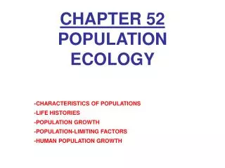
CHAPTER 52 POPULATION ECOLOGY. -CHARACTERISTICS OF POPULATIONS. -LIFE HISTORIES. -POPULATION GROWTH. -POPULATION-LIMITING FACTORS. -HUMAN POPULATION GROWTH.

E N D
CHAPTER 52POPULATION ECOLOGY -CHARACTERISTICS OF POPULATIONS -LIFE HISTORIES -POPULATION GROWTH -POPULATION-LIMITING FACTORS -HUMAN POPULATION GROWTH
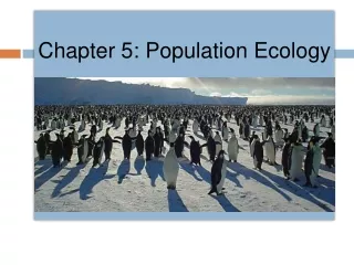
The size and activities of the human population are now among Earth’s most significant problems. With a population of over 6 billion individuals, our species requires vast amounts of materials and space, including places to live, land to grow our food, and places to dump our waste. Endlessly expanding our presence on Earth, we have devastated the environment for many other species and now threaten to make it unfit for ourselves . To understand human population growth, we must consider the general principles of population ecology. It is obvious that no population can continue to grow indefinitely. Species other than humans sometimes exhibit population explosions, but their populations inevitably decline. In contrast to these radical booms and busts, many populations are relatively stable over time, with only minor changes in population size . In our earlier study of biological populations (see Chapter 23), we emphasized the relationship between population genetics--the structure and dynamics of gene pools--and evolution. Evolution remains our central theme as we now view populations in the context of ecology. Population ecology, the subject of this chapter, is concerned with measuring changes in population size and composition, and with identifying the ecological causes of these fluctuations. Later in this chapter, we will return to our discussion of the human population. Let’s first examine some of the structural and dynamic aspects of populations as they apply to any species, such as the monarch butterfly population in the photo on this page .
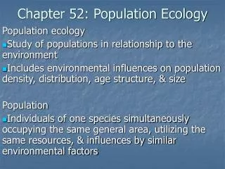
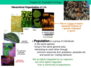
CHARACTERISTICS OF POPULATIONS Apopulation is a group of individuals of a single species that simultaneously occupy the same general area. They rely on the same resources, are influenced by similar environmental factors, and have a high likelihood of breeding with and interacting with one another. The characteristics of a population are shaped by interactions between individuals and their environments, and natural selection can modify these characteristics.
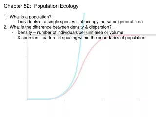
Two important characteristics of any population are density and the spacing of individuals At any given moment, every population has geographic boundaries and a population size (the number of individuals it includes). Ecologists begin studying a population by defining boundaries appropriate to the organisms under study and to the questions being posed. A population’s boundaries may be natural ones, such as a specific island in Lake Superior where terns nest, or they may be arbitrarily defined by an investigator, such as the oak trees within a specific county in Minnesota. Regardless of such differences, two important characteristics of any population are its density and its dispersion. Population density is the number of individuals per unit area or volume--the number of oak trees per square kilometer in the Minnesota county, for example. Dispersion is the pattern of spacing among individuals within the geographic boundaries of the population.
Measuring Density In rare cases, it is possible to determine population size and density by actually counting all individuals within the boundaries of the population. We could count the number of sea stars in a tide pool, for example. Herds of large mammals, such as buffalo or elephants, can sometimes be counted accurately from airplanes. In most cases, however, it is impractical or impossible to count all individuals in a population. Instead, ecologists use a variety of sampling techniques to estimate densities and total population sizes. For example, they might estimate the number of alligators in the Florida Everglades by counting individuals in a few randomly chosen plots. Or they might count the numbers of oak trees in several randomly placed circular plots of 10-m diameter. Such estimates are more accurate when there are many sample plots and when the habitat is homogeneous. Aerial census for African buffalo (Syncerus caffer) in the Serengeti of East Africa. Biologists can count large mammals and birds in open habitats from the air, either directly or from photographs like this one. By repeating these counts over many years, researchers can track population trends.
One sampling technique researchers often use to estimate fish and wildlife populations is the mark-recapture method. Traps are placed within the boundaries of the study area, and captured animals are marked with tags, collars, bands, or spots of dye and then immediately released. After a few days or a few weeks--enough time for the marked animals to mix randomly with unmarked members of the population--traps are set again. The proportion of marked (recaptured) animals in the second trapping is assumed equivalent to the proportion of marked animals in the total population: Thus, if there have been no births, deaths, immigration, or emigration, the following proportionality provides an estimate of the population size N : For example, suppose that 50 snowshoe hares are captured in box traps, marked with ear tags, and released. Two weeks later, 100 hares are captured and checked for ear tags. If 10 hares in this second catch are already marked and thus are recaptures, we would estimate that 10% of the total hare population is marked. Since 50 hares were originally marked, the entire population would be about 500 hares. This method assumes that each marked individual has the same probability of being trapped as each unmarked individual. This is not always a safe assumption, however. An animal that has been caught once may become wary of the traps later on or may learn to return to traps to eat the food used as bait.
In some cases, instead of counting individual organisms, population ecologists estimate density from some index of population size. This usually involves counting signs left by organisms, such as the number of nests, burrows, tracks, or fecal droppings.
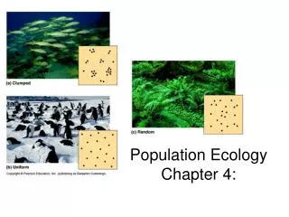
Patterns of Dispersion Within a population’s geographic range, local densities may vary substantially because the environment is patchy (not all areas provide equally suitable habitat) and because individuals exhibit patterns of spacing in relation to other members of the population.
The most common pattern of dispersion is clumped, with the individuals aggregated in patches. Plants may be clumped in certain sites where soil conditions and other environmental factors favor germination and growth. The eastern red cedar is often found clumped on limestone outcrops, where soil is less acidic than in nearby areas. Mushrooms may be clumped on a rotting log. Some animals move in herds. Animals often spend much of their time in a particular micro-environment that satisfies their requirements. For example, many forest insects and salamanders are clumped under logs, where the humidity remains high. Herbivorous animals of a particular species are likely to be most abundant where their food plants are concentrated. Clumping of animals may also be associated with mating behavior. For example, mayflies often swarm in great numbers, a behavior that increases mating chances for these insects, which spend only a day or two as reproductive adults. There may also be "safety in numbers"; fish swimming in large schools, for example, are often less likely to be eaten by predators than fish swimming alone or in small groups.
In contrast to a clumped distribution of individuals within a population, a uniform, or evenly spaced, pattern of dispersion may result from direct interactions between individuals in the population. For example, a tendency toward regular spacing of plants may be due to shading and competition for water and minerals; some plants also secrete chemicals that inhibit the germination and growth of nearby individuals that could compete for resources. Animals often exhibit uniform dispersion as a result of territorial behavior and aggressive social interactions. Uniform patterns are not as common in populations as clumped patterns.
Randomspacing (unpredictable dispersion) occurs in the absence of strong attractions or repulsions among individuals of a population; the position of each individual is independent of other individuals. For example, trees in a forest are sometimes randomly distributed. Random patterns are not as common in nature as one might expect; most populations show at least a tendency toward a clumped distribution.
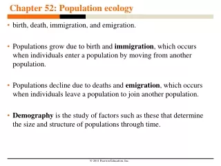
Demography is the study of factors that affect the growth and decline of populations Changes in population size reflect the relative rates of processes that add individuals to the population and eliminate individuals from it. Additions occur through births (which we will define here to include all forms of reproduction) and immigration, the influx of new individuals from other areas. Opposing these additions are mortality (death) and emigration, the movement of individuals out of a population. Our focus in this chapter is primarily on factors that influence birth rates and death rates, but you should remember that immigration and emigration may also play a role in population dynamics. The study of the vital statistics that affect population size is called demography. Birth rates vary among individuals (specifically, among females) within a population, depending, in particular, on age; and death rates depend on both age and sex. Let’s see how these demographic variables affect population dynamics.
Life Tables and Survivorship Curves About a century ago, when life insurance first became available, insurance companies developed an interest in the mathematics of survival. They needed to estimate how long, on average, an individual of a given age could be expected to live. Some of the greatest demographers of the past century worked for life insurance companies. They invented demographic representations called life tables. A life table is an age-specific summary of the survival pattern of a population. Population ecologists adapted this approach for nonhuman populations and developed quantitative demography as a branch of biology. The best way to construct a life table is to follow the fate of a cohort, a group of individuals of the same age, from birth until all are dead. The table is constructed from the number of individuals that die in each age-group during the defined time period. Cohort life tables are difficult to collect on wild animals and plants and are available only for a limited number of species. This is a life table for a cohort of Belding ground squirrels (Spermophilus beldingi ) at Tioga Pass, in California. Much can be learned about a population from a life table. The third column in the table shows the proportion of individuals in a cohort that are still alive at a given age. Notice that the death rates are generally highest among the youngest ground squirrels and among the oldest individuals and that males suffer higher rates of loss than females.
A graphic way of representing the data in a life table is to draw a survivorship curve, a plot of the proportion or numbers in a cohort still alive at each age. Survivorship curves can be classified into three general types. A Type I curve is relatively flat at the start, reflecting low death rates during early and middle life, then drops steeply as death rates increase among older age-groups. Humans and many other large mammals that produce relatively few offspring but provide them with good care often exhibit this kind of curve. In contrast, a Type III curve drops sharply at the left of the graph, reflecting very high death rates for the young, but then flattens out as death rates decline for those few individuals that have survived to a certain critical age. This type of curve is usually associated with organisms that produce very large numbers of offspring but provide little or no care, such as many fishes and marine invertebrates. An oyster, for example, may release millions of eggs, but most offspring die as larvae from predation or other causes. Those few that manage to survive long enough to attach to a suitable substrate and begin growing a hard shell, however, will probably survive for a relatively long time. Type II curves are intermediate, with a constant death rate over the life span. This kind of survivorship occurs in some annual plants, various invertebrates such as Hydra , some lizard species, and some rodents, such as the gray squirrel.
Many species, of course, fall somewhere between these basic types of survivorship or show more complex patterns. In birds, for example, mortality is often high among the youngest individuals (as in a Type III curve) but fairly constant among adults (as in a Type II curve). Some invertebrates, such as crabs, may show a "stair-stepped" curve, with brief periods of increased mortality during molts (caused by physiological problems or greater vulnerability to predation), followed by periods of lower mortality (when the exoskeleton is hard). In populations without immigration or emigration, survivorship is one of the two key factors determining changes in population size. Next we consider reproductive output, the other key factor determining population trends. Idealized survivorship curves. As an example of a Type I curve, humans in developed countries experience high survival rates until old age. At the opposite extreme are Type III curves for organisms such as oysters, which experience very high mortality as larvae but decreased mortality later in life. Type II survivorship curves are intermediate between the other two types and result when a constant proportion of individuals die at each age. Notice that the y axis is logarithmic and that the x axis is on a relative scale, so that species with widely varying life spans can be compared on the same graph.
Reproductive Rates Demographers who study sexually reproducing species generally ignore males and concentrate on females in the population because only females give birth to offspring. Demographers view populations in terms of females giving rise to new females; males are important only as distributors of genes. How can we describe the reproductive program of a population? The simplest way is to follow the basic approach of the life table and ask how reproductive output varies with age.
A reproductive table, or fertility schedule, is an age- specific summary of the reproductive rates in a population. The best way to construct a fertility schedule is to measure the reproductive output of a cohort from birth until death. For sexual species, the reproductive table tallies the number of female offspring produced by each age-group. The table below illustrates a reproductive table for Belding ground squirrels. Reproductive output for sexual species like birds and mammals is a product of the fraction of females of a given age that are breeding and the number of female offspring of those breeding females. By multiplying these together, we can obtain the average output of daughters for each individual in a given age class (the last column). For these ground squirrels, which begin to reproduce at age 1 year, reproductive output rises to a peak at 4 years of age and then falls off in older females.
Reproductive tables vary greatly, depending on the species. Squirrels have a litter of two to six young once a year, whereas oak trees drop thousands of acorns each year for tens or hundreds of years. Salmon lay thousands of eggs when they spawn, and mussels and other invertebrates may release hundreds of thousands of eggs in a spawning cycle. Why does one type of life cycle rather than another evolve in a particular population? This is one of the many questions at the interface of population ecology and evolutionary biology.
LIFE HISTORIES Natural selection will favor traits in organisms that improve their chances of survival and reproductive success. Organisms that survive a long time but do not reproduce are not at all "fit" in the Darwinian sense. In every species, there are trade-offs between survival and traits such as frequency of reproduction, investment in parental care, and the number of offspring produced (seed crops for seed plants and litter size or clutch size for animals). The traits that affect an organism’s schedule of reproduction and survival (from birth through reproduction to death) make up its life history. Of course, a particular life history, like most characteristics of an organism, is the result of natural selection operating over evolutionary time. Life history traits help determine how populations grow.
Life histories are highly diverse, but they exhibit patterns in their variability Because of varying environmental contexts for natural selection, life histories are very diverse. Pacific salmon, for example, hatch in the headwaters of a stream, then migrate to open ocean, where they require one to four years to mature. They eventually return to freshwater streams to spawn, producing thousands of small eggs in a single reproductive opportunity, and then they die. Ecologists call this big-bang reproduction. This figure illustrates big-bang reproduction in agaves. The agave, or century plant, grows in arid climates with sparse and unpredictable rainfall. Agaves grow vegetatively for several years, then send up a large flowering stalk, produce seeds, and die. (We introduced the big-bang reproduction of century plants on the opening page of Chapter 38.) The shallow roots of agaves catch water after rain showers but are dry during droughts. This unpredictable water supply may prevent seed production or seedling establishment for several years at a time. By growing and storing nutrients until an unusually wet year and then putting all its resources into reproduction, the agave’s big-bang strategy is a life history adaptation to erratic climate. In another example of big-bang reproduction, annual desert wildflowers generally germinate, grow, produce many small seeds, and then die, all in the span of a month after spring rains. Big-bang (one-time) reproduction is also called semelparity(from the Latin semel , once, and parito , to beget). An example of big-bang reproduction. Agaves, or century plants, grow without reproducing for several years and then produce a gigantic flowering stalk and many seeds. After this onetime reproductive effort, the plant dies.
In contrast to big-bang reproduction, some lizards produce only a few large eggs during their second year of life, then repeat the reproductive act annually for several years. And some species of oaks do not reproduce until the tree is 20 years old, but then produce vast numbers of large seeds each year for a century or more. Ecologists call this repeated reproduction or iteroparity (from the Latin itero , to repeat). What factors contribute to the evolution of semelparity versus iteroparity? That is, how much will an individual gain in reproductive success through one strategy versus the other? The key demographic effect of big-bang reproduction is higher reproductive rates. Plants like agaves that reproduce only once typically produce two to five times as many seeds as closely related species that reproduce repeatedly. The critical factor in the evolutionary dilemma of big-bang versus repeated reproduction is the survival rate of the offspring. If their chance of survival is poor or inconsistent, repeated reproduction will be favored.
Limited resources mandate trade-offs between investments in reproduction and survival Darwinian fitness is measured not by how many offspring are produced but by how many survive to produce their own offspring: Heritable characteristics of life history that result in the most reproductively successful descendants will become more common within the population. If we were to construct a hypothetical life history that would yield the greatest lifetime reproductive output, we might imagine a population of individuals that begin reproducing at an early age, produce many offspring each time they reproduce, and reproduce many times in a lifetime. However, natural selection cannot maximize all these variables simultaneously, because organisms have finite resources, and limited resources mean trade-offs. Ecologists who study the evolution of life histories focus on how these trade-offs operate in specific populations. For example, the production of many offspring with little chance of survival may result in fewer descendants than the production of a few well-cared-for offspring that can compete vigorously for limited resources in an already dense population.
The life histories we observe in organisms represent an evolutionary resolution of several conflicting demands. Time, energy, and nutrients that are used for one thing cannot be used for something else. In the broadest sense, there is a trade-off between reproduction and survival, and this has been demonstrated by several studies. For example, in red deer on the Scottish island of Rhum, females that reproduce in one summer suffer higher mortality over the following winter than do females that did not reproduce. This cost of reproduction was found even in red deer in the prime of life, but was particularly severe in the older females. And in many insect species, females that lay fewer eggs live longer, suggesting a similar trade-off between investing in current reproduction and survival. Cost of reproduction in female red deer on the island of Rhum, in Scotland. Mortality in winter is higher for females that reproduced during the previous summer, no matter what the age of the female.
There can also be trade-offs between current and future reproduction. When perennial plants produce more seeds in one year, they grow less and have reduced seed production the next year. Moreover, experimental transfers of eggs or nestlings in bird populations have measured the trade-off between reproductive effort and survival. When nestlings of European kestrels were transferred among nests to produce broods of three or four (reduced), five or six (normal), and seven or eight (enlarged), adult kestrels that raised the enlarged broods survived poorly over the following winter. Probability of survival over the following year for European kestrels after raising a modified brood. A total of 200 birds were studied from 1985 to 1990 in the Netherlands. Adults with experimentally enlarged broods die more often over the following winter. (Both males and females provide parental care for the nestlings.)
As in our red deer and kestrel examples, many life history issues involve balancing the profit of immediate investment in offspring against the cost to future prospects of survival and reproduction. These issues can be summarized by three basic "decisions": when to begin reproducing, how often to breed, and how many offspring to produce during each reproductive episode. The various "choices" are integrated into the life history patterns we see in nature. It is important to clarify our use of the word choice . Organisms do not choose consciously when to breed and how many offspring to have. (Humans are an important exception we will consider later in the chapter.) Life history traits are evolutionary outcomes reflected in the development, physiology, and behavior of an organism. Age at maturity and the number of offspring produced during a given reproductive episode are usually maintained within narrow ranges by stabilizing selection. Natural selection molds reproductive patterns in populations; such patterns are not consciously chosen by the organism.
As with all life history adaptations, the number and size of offspring depend on the selective pressures under which the organism evolved. Plants and animals whose young are subject to high mortality rates often produce large numbers of relatively small offspring. Thus, plants that colonize disturbed environments usually produce many small seeds, most of which will not reach a suitable environment. Small size might actually benefit such seeds if it enables them to be carried long distances. Birds and mammals that suffer high predation rates also produce large numbers of offspring; examples include quail, rabbits, and mice. Variation in seed crop size in plants. Most weedy plants, such as this dandelion, grow quickly and produce a large number of seeds. Although most of the seeds will not produce mature plants, their large number and ability to disperse to new habitats ensure that at least some will grow and eventually produce seeds themselves.
In other organisms, extra investment on the part of the parent greatly increases the offspring’s chances of survival. Oak, walnut, and coconut trees all have large seeds with a large store of energy and nutrients that the seedlings can use to become established. In animals, parental investment in offspring does not always end with incubation or gestation. Primates generally have only one or two offspring at a time. Parental care and an extended period of learning in the first several years of life are very important to offspring fitness in these mammals. Now that we have analyzed some patterns that underlie diverse life histories, let’s examine the effects of these life history traits on the growth of populations. Variation in seed crop size in plants. Some plants, such as this coconut palm, produce a moderate number of very large seeds. The large endosperm provides nutrients for the embryo (a plant’s version of parental care), an adaptation that helps ensure the success of a relatively large fraction of offspring. Animal species exhibit similar trade-offs between number of offspring and the amount of nutrients provided to each offspring.
POPULATION GROWTH To begin to understand the potential for population increase, consider a single bacterium that can reproduce by fission every 20 minutes under ideal laboratory conditions. At the end of this time, there would be two bacteria, four after 40 minutes, and so on. If this continued for only a day and a half--a mere 36 hours--there would be enough bacteria to form a layer a foot deep over the entire Earth. At the other life history extreme, elephants may produce only six young in a 100-year life span. Still, Darwin calculated that it would take only 750 years for a single pair of elephants to produce a population of 19 million. Obviously, indefinite population increase does not occur for any species, either in the laboratory or in nature. A population that begins at a low level in a favorable environment may increase rapidly for a while, but eventually the numbers must, as a result of limited resources and other factors, stop growing.
As we discussed in Chapter 50, finding the answers to ecological questions depends on a combination of observation and experimentation. The two major forces affecting population growth--birth rates and death rates--can be measured in many populations and used to predict how the populations will change in size over time. Small organisms can be studied in the laboratory to determine how various factors affect their population growth rates, and natural populations can be experimentally manipulated to answer the same questions. Mathematical models can be used for testing hypotheses about the effects of different factors on population growth once we understand how birth and death rates change over time. We can begin to understand population growth by looking at a few simple models of how a population can grow.
The exponential model of population growth describes an idealized population in an unlimited environment Imagine a hypothetical population consisting of a few individuals living in an ideal, unlimited environment. Under these conditions, there are no restrictions on the abilities of individuals to harvest energy, grow, and reproduce, aside from the inherent physiological limitations that are the result of their life history. The population will increase in size with every birth and with the immigration of individuals from other populations and decrease in size with every death and with the emigration of individuals out of the population. For simplicity, let’s ignore the effects of immigration and emigration (a more complex formulation would certainly include these factors). We can define a change in population size during a fixed time interval with the following verbal equation: Using mathematical notation, we can express this relationship more concisely. If N represents population size and t represents time, then ΔN is the change in population size and Δt is the time interval (appropriate to the life span or generation time of the species) over which we are evaluating population growth. (The Greek letter delta, Δ, indicates change, such as change in time.) We can now rewrite the verbal equation as where B is the number of births in the population during the time interval and D is the number of deaths. Similarly, the per capita death rate, symbolized as d , allows us to calculate the expected number of deaths per unit time in a population of any size. If d = 0.016 per year, we would expect 16 deaths per year in a population of 1,000 individuals. (Using the formula D = dN , how many deaths would you expect per year if d = 0.010 annually in populations of 500, 700, and 1,700?) For natural populations or those in the laboratory, the per capita birth rates and death rates can be calculated from estimates of population size and data given in life tables and reproductive tables.
We can revise the population growth equation again, this time using per capita birth rates and death rates rather than the numbers of births and deaths: One final simplification is in order. Population ecologists are concerned with overall changes in population size, using r to identify the difference in the per capita birth rates and death rates: This value, the per capita growth rate, tells whether a population is actually growing (positive value of r ) or declining (negative value of r ). Zero population growth (ZPG) occurs when the per capita birth rates and death rates are equal (r = 0). Note that births and deaths still occur in the population, but they balance each other exactly. (Later in this chapter, we will discuss the relevance of ZPG for the human population and the factors preventing the human population from leveling off.) Using the per capita growth rate, we rewrite the equation for change in population size as Finally, most ecologists use the notation of differential calculus to express population growth in terms of instantaneous growth rates: If you have not yet studied calculus, don’t be intimidated by the form of the last equation; it is essentially the same as the previous one, except that the time intervals Δt are very short and are expressed in the equation as dt . (Do not confuse this use of d to symbolize very small change with our earlier use of d to represent per capita death rate.)
We started this section by describing a population living under ideal conditions, where organisms are constrained only by their life history. In such a situation, the population grows rapidly, because all members have access to abundant food and are free to reproduce at their physiological capacity. Population increase under these ideal conditions is called exponential population growth, or geometric population growth. Under these conditions the per capita growth rate may assume the maximum growth rate for the species, called the intrinsic rate of increase, denoted as rmax . And the equation for exponential population growth is then: The size of a population that is growing exponentially increases rapidly, resulting in a J-shaped growth curve when population size is plotted over time. Although the intrinsic rate of increase is constant as the population grows, the population actually accumulates more new individuals per unit of time when it is large than when it is small; thus, the curves in FIGURE 52.8 get progressively steeper over time. This occurs because population growth depends on N as well as r , and larger populations experience more births (and deaths) than small ones growing at the same per capita rate. It is also clear from FIGURE 52.8 that a population with a higher intrinsic rate of increase (dN/dt = 1.0N ) will grow faster than one with a lower rate of increase (dN/dt 5 = 0.5N ). Population growth predicted by the exponential model. The exponential growth model predicts unlimited population increase under conditions of unlimited resources. This graph compares growth in populations with two different values of r : 1.0 and 0.5.
The J-shaped curve of exponential growth is characteristic of some populations that are introduced into a new or unfilled environment or whose numbers have been drastically reduced by a catastrophic event and are rebounding. For example, this figure illustrates exponential population growth in the whooping crane, an endangered species now recovering from the impact of habitat loss due to agriculture. Example of exponential population growth in nature. The whooping crane is an endangered species that has been recovering from near extinction since 1940. Counts of adults are made annually on the wintering grounds at Aransas, Texas. In the year 2000-2001, there were 179 birds in the wintering population in Texas, the population having declined slightly from the preceding year. The overall average rate of increase has been 4% per year since the 1950s.
The logistic model of population growth incorporates the concept of carrying capacity The exponential growth model assumes unlimited resources, which is never the case in the real world. No population--neither bacteria nor elephants nor any other organisms--can grow exponentially indefinitely. As any population grows larger in size, its increased density may influence the ability of individuals to harvest sufficient resources for maintenance, growth, and reproduction. Populations subsist on a finite amount of available resources, and as the population becomes more crowded, each individual has access to an increasingly smaller share. Ultimately, there is a limit to the number of individuals that can occupy a habitat. Ecologists define carrying capacity as the maximum population size that a particular environment can support at a particular time with no degradation of the habitat. Carrying capacity, symbolized asK, is not fixed, but varies over space and time with the abundance of limiting resources. For example, the carrying capacity for bats may be high in a habitat where flying insects are abundant and there are caves for roosting but lower in a habitat where food is abundant but suitable shelters are less common. Energy limitation is one of the most significant determinants of carrying capacity, although other factors, such as shelters, refuges from predators, soil nutrients, water, and suitable nesting and roosting sites, can be limiting.
Crowding and resource limitation can have a profound effect on the population growth rate. If individuals cannot obtain sufficient resources to reproduce, per capita birth rate will decline. If they cannot find and consume enough energy to maintain themselves, per capita death rates may also increase. A decrease in b or an increase in d results in a smaller r and a lower overall rate of population growth. Yellow bacterial colonies with EPS of Xanthomonas campestris pv. vesicatoria grown on sucrose-peptone-agar medium
The Logistic Growth Equation We can modify our mathematical model of population growth to incorporate changes in growth rate as the population size nears the carrying capacity (as N grows toward K ). The logistic population growth model incorporates the effect of population density on the per capita rate of increase, allowing this rate to vary from a maximum at low population size to zero as carrying capacity is reached. When a population’s size is below the carrying capacity, population growth is rapid, but as N approaches K , population growth slows down.
Mathematically, we construct the logistic model by starting with the model of exponential population growth and creating an expression that reduces the rate of population increase as N increases. If the maximum sustainable population size is K , then K -N tells us how many additional individuals the environment can accommodate, and (K -N )/K tells us what fraction of K is still available for population growth. By multiplying the exponential rate of increase rmaxN by (K -N )/K , we reduce the actual growth rate of the population as N increases: Reduction of population growth rate with increasing population size (N ). The logistic model of population growth assumes that the population growth rate dN/dt decreases as N increases. When N is close to 0, the population grows rapidly. However, as N approaches K (the carrying capacity of the environment), the population growth rate approaches 0, and population growth slows. If N is greater than K , then the population growth rate is negative, and population size decreases. An equilibrium is reached at the white line when N = K .
The table below shows hypothetical calculations for the rate of population increase and changes in N at various population sizes for a population growing according to the logistic model. Notice that when N is small compared to K , the term (K -N )/K is large, and the actual rate of population increase (dN/dt ) is close to the intrinsic (maximum) rate of increase. But when N is large and resources are limiting, then (K -N )/K is small, and so is the rate of population increase. Zero population growth occurs when the numbers of births and deaths are equal--when N equals K .
The logistic model of population growth produces a sigmoid (S-shaped) growth curve when N is plotted over time. New individuals are added to the population most rapidly at intermediate population sizes, when there is not only a breeding population of substantial size, but also lots of available space and other resources in the environment. The population growth rate slows dramatically as N approaches K . Notice that we haven’t said anything about what makes the population growth rate change as N approaches K . Either the birth rate b must decrease, the death rate d must increase, or both. Later in the chapter, we will go into some detail about some of the factors affecting b and d . Population growth predicted by the logistic model. The logistic growth model assumes that there is a maximum population size that the environment can support--the carrying capacity K . The rate of population growth slows as the population approaches the carrying capacity of the environment. The red line shows logistic growth in a population where rmax = 1.0 and K = 1,500 individuals. For comparison, the blue line illustrates a population continuing to grow exponentially with the same rmax .
How Well Does the Logistic Model Fit the Growth of Real Populations? The growth of laboratory populations of some small animals, such as beetles or crustaceans, and of microorganisms, such as paramecia, yeasts, and bacteria, fit S-shaped curves fairly well (FIGURE a). These experimental populations are grown in a constant environment lacking predators and other species that may compete for resources, conditions that rarely occur in nature. Even under these laboratory conditions, not all populations show logistic growth patterns. Laboratory populations of water fleas (Daphnia ) , for example, show exponential growth and overshoot their carrying capacity before settling down to a relatively stable density (FIGURE b). Most populations show some deviations from a smooth sigmoid curve. And while many natural populations increase in approximately logistic fashion, the stable carrying capacity is rarely observed. FIGURE c shows population changes in the song sparrow on a small island in southern British Columbia. The population increases rapidly but suffers periodic catastrophes in winter, so that there is no stable population size. How well do these populations fit the logistic population growth model? The dots on these graphs are the actual data points.
Some of the basic assumptions built into the logistic model clearly do not apply to all populations. For example, the model incorporates the idea that even at low population levels, each individual added to the population has the same negative effect on population growth rate. Some populations, however, show an Allee effect (named after W. C. Allee, of the University of Chicago, who first described it), in which individuals may have a more difficult time surviving or reproducing if the population size is too small. For example, a single plant standing alone may suffer from excessive wind but would be protected in a clump of individuals. And some seabirds that breed in colonies require large numbers at their breeding grounds to provide the necessary social stimulation for reproduction. Moreover, conservation biologists fear that populations of solitary animals, such as rhinoceroses, may become so small that individuals will not be able to locate mates in the breeding season. In all these cases, a greater number of individuals in the population has a positive effect, up to a point, on population growth, rather than a negative effect as assumed by the logistic model.
The logistic model also makes the assumption that populations adjust instantaneously and approach carrying capacity smoothly. In most natural populations, however, there is a lag time before the negative effects of an increasing population are realized. For example, as some important resource, such as food, becomes limiting for a population, reproduction will be reduced, but the birth rate may not be affected immediately because the organisms may use their energy reserves to continue producing eggs for a short time. This may cause the population to overshoot the carrying capacity. Eventually, deaths will exceed births, and the population may then drop below carrying capacity; even though reproduction begins again as numbers fall, there is a delay until new individuals actually appear. Many populations fluctuate strongly, which makes it difficult to define what is meant by carrying capacity (see FIGURE c). Others overshoot it at least once before attaining a relatively stable size (see FIGURE b). We will examine some possible reasons for these fluctuations later in the chapter.
As you will see in the next section, some populations do not necessarily remain at, or even reach, levels where population density is an important factor. In many insects and other small, quickly reproducing organisms that are sensitive to environmental fluctuations, physical variables such as temperature or moisture usually reduce the population well before resources become limiting. Overall, the logistic model is a useful starting point for thinking about how populations grow and for constructing more complex models. Although it fits few, if any, real populations closely, the logistic model is useful in conservation biology and in pest control to estimate how rapidly a particular population might increase in numbers after it has been reduced to a small size. And like any good starting hypothesis, the logistic model has stimulated much research and many discussions that, whether they support the model or not, lead to a greater understanding of the factors affecting population growth. Female with ootheca (egg case)
The Logistic Population Growth Model and Life Histories The logistic model predicts different growth rates for low-density populations and high-density populations, relative to the carrying capacity of the environment. At high densities, each individual has few resources available, and the population can grow slowly, if at all. At low densities, the opposite is true: Resources per capita are relatively abundant, and the population can grow rapidly. Different life history features will be favored under these different conditions. At high population density, selection favors adaptations that enable organisms to survive and reproduce with few resources. Thus, competitive ability and maximum efficiency of resource utilization should be favored in populations that are at or near their carrying capacity. At low population density, on the other hand, even in the same species, the "empty" environment should favor adaptations that promote rapid reproduction. Increased fecundity and earlier maturity, for example, would be selected for.
Thus, the life history traits that natural selection favors may vary with population density and environmental conditions. Selection for life history traits that are sensitive to population density can be called K -selection, or density-dependent selection. In contrast, selection for life history traits that maximize reproductive success in uncrowded environments (low densities) can be called r -selection, or density-independent selection. These names follow from the variables of the logistic equation. K -selection tends to maximize population size and operates in populations living at a density near the limit imposed by their resources (the carrying capacity K ). By contrast, r -selection tends to maximize r , the rate of increase, and occurs in variable environments in which population densities fluctuate well below carrying capacity or in open habitats where individuals are likely to face little competition.
In laboratory experiments, researchers have shown that different populations of the same species may show a different balance of K -selected and r -selected traits, depending on conditions. For example, cultures of the fruit fly Drosophila melanogaster raised under crowded conditions with minimal food for 200 generations are more productive at high density than populations raised in uncrowded conditions with maximal food. Larvae from cultures selected for living in crowded conditions feed faster than larvae selected for living in uncrowded cultures. The fruit fly genotypes that are most fit at low density do not have high fitness at high density, as predicted by r- and K - selection theory.
POPULATION-LIMITING FACTORS There are two general questions that we can ask about population growth. First, why do all populations eventually stop increasing? Exponential population growth is rare in nature and always of short duration. What environmental factors stop a population from growing? If we have an introduced weed that is spreading rapidly, what should we do to stop its population growth? Second, why is the population density of a particular species greater in some habitats than in others? Every bird-watcher can tell you what the favorable and unfavorable habitats are for any particular bird species. What determines a favorable habitat, and how do we turn an unfavorable habitat into a good one?
These questions have many practical applications. A conservation biologist might want to turn a declining species population into an increasing one. And in agriculture, the objective may be to get a pest population to decrease. Moreover, agricultural pests may have severe effects in some areas and negligible effects in others. Why? Endangered species, meanwhile, such as humpback whales, require good habitats for survival. What environmental factors create a favorable feeding habitat for humpbacks? All these practical issues involve population-limiting factors. Regulation is one of this book’s ten themes (see Chapter 1). In this section, we apply that theme to populations.
The first step in understanding why a population stops growing is to find out how the rates of birth, death, immigration, and emigration change as population density rises. If immigration and emigration offset each other, then a population grows when the birth rate exceeds the death rate and declines when the death rate exceeds the birth rate. This graph shows a simple graphical model of how a population may stop increasing and reach equilibrium. A death rate that rises as population density rises is said to be density dependent, as is a birth rate that falls with rising density. Density-dependent rates are an example of negative feedback, a type of regulation you learned about in Chapter 1. In contrast, a birth rate or death rate that does not change with population density is said to be density independent. With density-independent rates, there is no feedback to slow down population growth. Graphic model showing how equilibrium may be determined for population density. Population density reaches equilibrium only when the per capita birth rate equals the per capita death rate, and this is possible only if the birth or death rate (or both) changes with density (is a density-dependent rate). In this simple model, immigration and emigration are assumed to be either zero or equal.
Negative feedback prevents unlimited population growth No population stops growing without some type of negative feedback between population density and the vital rates of birth and death. Once we know how birth and death rates change with population density, we need to determine the mechanisms causing these changes. Because populations are affected by a variety of factors that cause negative feedback, it can be a challenge to pinpoint the exact factors at work in a particular population. Although field studies may eventually shed light on the most important factors producing negative feedback in specific cases, they have not yet provided many generalizations. First, much of the research on populations has been conducted in the temperate zone, and we need many more studies of tropical and polar organisms to complete the picture. Second, birds and mammals have been the subjects of much more research than have other organisms. In particular, insects, which form the dominant group of species on Earth, have not been studied in proportion to their species’ richness. Finally, long time periods are required for experimental work on population dynamics, with definitive studies routinely taking 10 to 20 years for completion. With these reservations in mind, let us look at several examples of how birth and death rates change with population density--in some cases where the mechanisms behind these changes are well understood.