Download
1 / 78
850 likes | 1.33k Vues
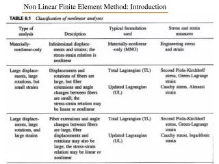
Introduction to Finite Element Modeling in Biomechanics. Dr. N. Fatouraee Biomedical Engineering Faculty December, 2004. Overview. Introduction and Definitions Basic finite element methods 1-D model problem Application Examples. Overview. Finite Element Method

E N D
Introduction to Finite Element Modeling in Biomechanics Dr. N. Fatouraee Biomedical Engineering Faculty December, 2004
Overview • Introduction and Definitions • Basic finite element methods • 1-D model problem • Application Examples
Overview • Finite Element Method • numerical method to solve differential equations E.g.: Flow Problem u(r) Heat Transfer Problem T(r,t)
The “Continuum” Concept • biomechanics example: blood flow through aorta • diameter of aorta 25 mm • diameter of red blood cell 8 m (0.008 mm) • treat blood as homogeneous and ignore cells
The “Continuum” Concept • biomechanics example: blood flow through capillaries • diameter of capillary can be 7 m • diameter of red blood cell 8 m • clearly must include individual blood cells in model
Continuous vs. Discrete Solution • What if the equation had no “analytical solution” (e.g., due to nonlinearities)?
Continuous vs. Discrete Solution • What if the equation had no “analytical solution” (e.g., due to nonlinearities)? • How would you solve an ordinary differential equation on the computer? • Numerical methods • Runge-Kutta • Euler method
Discretization 0 1 0 1
0 1 Discretization in general, Euler method is given by: • Start with initial condition: y(x0)=y0 • Calculate f(x0,y0) • Calculate y1=y0 + f(x0,y0) x • Calculate f(x1,y1) …………..
y Exact Solution 8 Steps 4 Steps 2 Steps x Euler Example ODE: dy/dx (x,y) = 0.05 yInitial Cond.: y(0)=100 Problem: Use Euler with 2 steps: Calculate y(x) between at x=20 and x=40 Euler, 2 steps: dy/dt(0,100) = 5 ; x = 20 y(20) = y(0) + x*dy/dt(0,100) = 100 + 20*5= 200 y(40) = y(20) + x*dy/dt(20,200) = 200 + 20* 10 = 400
Discretization • in general, the process by which a continuous, differential equation is transformed into a set of algebraic equations to be solved on a computer • various forms of discretization • finite element, finite difference, finite volume
Finite Element Method • discretization • steps in finite element method • weak form of differential equation • interpolation functions within elements • solution of resulting algebraic equations
Basic Finite Element Methods:A 1-D Example solve for u(x)
Basic Finite Element Methods:A 1-D Example Note that for a=0, b=1:
Basic Finite Element Method • seek solution to allied formulation referred to as “weak” statement
Basic Finite Element Method • seek solution to allied formulation referred to as “weak” statement
Basic Finite Element Method The integral form is as valid as the original differential equation.
Basic Finite Element Method note that by the chain rule:
Basic Finite Element Method note that by the chain rule:
Basic Finite Element Method recall: w(x) is arbitraryno loss in generality to require w(a)=w(b)=0 i.e., subject w to same boundary conditions as u
Basic Finite Element Method “weak statement”: the above expression is “continuous” i.e., must be evaluated for all x
Discretization 0 1 0 1 “elements” “nodes”
Discretization 1 2 3 4 5 6 “nodes” “elements” 1 2 3 4 5 u defined at nodes u1, u2 … = u(x1),u(x2) … goal solve for ui
Discretization 1 2 3 4 5 6 “nodes” “elements” 1 2 3 4 5
Consider a Typical Element e x2 x1
Interpolation Functions Within the element we interpolate between u1 and u2:
e x2 x1 Interpolation Functions at x = x1: u = u1 at x = x2: u = u2 x1 < x < x2: interpolation between u1 and u2 u1, u2 unknowns to be solved for i.e., nodal values of u
Approximation Functions Now we have to choose functions for w: - referred to as “Galerkin” method
We end up with a system of algebraic equations, that canbe solved by the computer
How many elements do we need? 0 1 1 2 3 4 5 6 “nodes” “elements” 1 2 3 4 5
5 elements 2 elements 20 elements 10 elements
Practical Finite Element Analysis • many commercial finite element codes exist for different disciplines • FIDAP, FLUENT: fluid mechanics • ANSYS, LS-Dyna, Abaqus: solid mechanics
Using a Commercial Code • choose most appropriate software for problem at hand • not always trivial • can the code handle the key physical processes • e.g., spatially varying material properties, nonlinearities
Steps in Finite Element Method (FEM) • Geometry Creation • Material properties (e.g. mass density) • Initial Conditions (e.g. temperature) • Boundary Conditions • Loads (e.g. forces) • Mesh Generation • Solution • Time discretization (for transient problems) • Adjustment of Loads and Boundary Conditions • Visualization • Contour plots (on cutting planes) • Iso surfaces/lines • Vector plots • Animations • Validation
Model Validation • most important part of the process, but hardest and often not done • two types of validation • code validation: are the equations being solved correctly as written (i.e., grid resolution, etc.) • model validation: is the numerical model representative of the system being simulated (very difficult)
Radiofrequency Ablation forLiver Cancer • Surgical Resection is currently the gold-standard, and offers 5-year survival of around 30% • Surgical Resection only possible in 10-20% of the cases • Radiofrequency Ablation heats up tissue by application of electrical current • Once tumor tissue reaches 50°C, cancer cells die
Electric Field Effects of RF energy on tissue • Electrical Current is applied to tissue • Electrical current causes heating by ionic friction • Temperatures above ~50 °C result in cell death (necrosis) Na+ K+ Cl- Cl- Cl- Na+
Clinical procedure Insertion Probe Extension • Ground pad placed on patients back or thighs • Patient under local anesthesia and conscious sedation, or light general anesthesia Application of RF power(~12-25 min)
Current RF Devices 200W RF-generator (Radionics / Tyco) 9-prong probe, 5 cm diameter, (Rita Medical) Cool-Tip probe, 17-gauge needle, (Radionics / Tyco) 12-prong probe,4 cm diameter,(Boston Scientific)
RF Lesion Pathology Coagulation Zone (= RF lesion, >50 °C) Hyperemic Zone (increased perfusion)
Finite Element Modeling for Radiofrequency Ablation • Purpose of Models: • Investigate shortcomings of current devices • Simulate improved devices • Estimate RF lesion dimensions for treatment planning • Thermo-Electrically Coupled Model: • Solve Electric Field problem (Where is heat generated) • Solve thermal problem (Heat Conduction in Tissue, Perfusion, Vessels)
Electric Field Problem (Where is heat being generated?) Laplace’s Equation Boundary Conditions P M Electric Field
Thermal Problem:Conservation of Energy rate of change of energy in a body = + rate of energy generation + rate of energy addition - rate of energy lost
energy transfer (“conducted”) to surrounding tissue energy transfer to blood flow carrying heat away (“convected”) energy transferred (“conducted”) back to electrode energy storage by tissue energy added due to metabolism energy added by electric current (Power = current*voltage)
1 cm Model Geometry 2-D axisymmetric model
Animations Electrical Current Density(Where is heat being generated?) Temperature