Download
1 / 61
610 likes | 727 Vues
This study focuses on the advancement of ensemble-based predictions and diagnostics in understanding tropical cyclone formation during the PREDICT field experiment. Recognizing that only about 20% of tropical waves evolve into depressions, this research investigates the physical differences between developing and non-developing systems, considering multi-scale processes like large-scale environments, wave structures, and convective-scale phenomena. The utility of ensemble forecasts across global, regional, and convective scales is explored, providing insights into critical values influencing cyclone genesis, such as relative vorticity and wind shear.

E N D
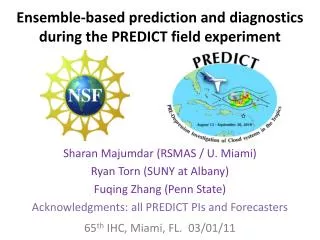
Ensemble-based prediction and diagnostics during the PREDICT field experiment Sharan Majumdar (RSMAS / U. Miami) Ryan Torn (SUNY at Albany) Fuqing Zhang (Penn State) Acknowledgments: all PREDICT PIs and Forecasters 65th IHC, Miami, FL. 03/01/11
The problem • Only ~20% of tropical waves develop into depressions. • Need to advance understanding of the physical differences between developing and non-developing systems. • Tropical cyclone formation is a multi-scale process, which depends on • Large-scale environment in which it is embedded • Wave’s structure (low-level vorticity, mid-level moisture) • Convective-scale processes: hot towers etc. • Seek to investigate utility of ensemble forecasts • Global; Regional; Convective-scale
Offer a longer-term outlook (>1 week) on the potential for a tropical disturbance to develop. • Scatter of forecasts depicting critical values of • Area-averaged vorticity • Geopotential thickness anomaly • Okubo-Weiss parameter • Probabilities of exceedanceof critical values of • Vertical wind shear • Lower-tropospheric relative humidity • Upper level divergence / lower-level convergence • Offer hypotheses on processes that lead to errors in large-scale conditioning (and thereby inaccurate representations of smaller-scale processes)
Example: Genesis of Karl (AL13; PGI44L) • Monsoon-like trough predicted to meander northward from the northern coast of South America into the southern Caribbean. • ECMWF ensemble forecasts of • (TOP) 700-850 hPa relative vorticity averaged over disk of radius 300 km • (BOTTOM) 200-850 hPa thickness anomaly: Z(r=250 km) – Z(r=1000 km) • All initialized on 00 UTC, 8 Sept 2010 • 7 days prior to genesis
Example: Genesis of Karl (AL13; PGI44L) • 7-day forecasts of • Probability that 700 hPa RH > 70% • Okubo-Weiss parameter (vorticity^2 – strain rate^2): indicator of strongly curved flow with minimum horizontal shearing deformation
Contours of O-W: 2 x 10⁻⁹ s-2 X X X X
Example: Genesis of Karl (AL13; PGI44L) • Genesis occurred just before 00 UTC, 15 Sep • Next two “loops” • 9- through 0- day ensemble forecasts of area-averaged relative vorticity valid at genesis time • Same but displayed as PDFs