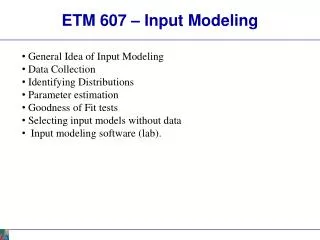
Input Modeling in Discrete-Event Simulation
Learn the steps of input model development, data collection techniques, identifying distributions, and fitting the chosen distribution. Explore histograms, selecting distribution families, and using Q-Q plots for evaluating the model fit. Enhance your input modeling skills!

Input Modeling in Discrete-Event Simulation
E N D
Presentation Transcript
Chapter 9 Input Modeling Banks, Carson, Nelson & Nicol Discrete-Event System Simulation
Purpose & Overview • Input models provide the driving force for a simulation model. • The quality of the output is no better than the quality of inputs. • In this chapter, we will discuss the 4 steps of input model development: • Collect data from the real system • Identify a probability distribution to represent the input process • Choose parameters for the distribution • Evaluate the chosen distribution and parameters for goodness of fit.
9.1 Data Collection One of the biggest tasks in solving a real problem. GIGO – garbage-in-garbage-out Examples • Stale data – different methods of collection • Unexpected data – metal detector delay • Time-varying data – camel hump call center • Dependent data – drinks in season
Data Collection - suggestions start on page 340 • Suggestions that may enhance and facilitate data collection: • Plan ahead: begin by a practice or pre-observing session, watch for unusual circumstances • Analyze the data as it is being collected: check adequacy • Combine homogeneous data sets, e.g. successive time periods, during the same time period on successive days • Be aware of data censoring: the quantity is not observed in its entirety, danger of leaving out long process times • Check for relationship between variables, e.g. build scatter diagram • Check for autocorrelation • Collect input data, not performance data
9.2 Identifying the Distribution • Histograms • Selecting families of distribution • Parameter estimation • Goodness-of-fit tests • Fitting a non-stationary process
Histograms [Identifying the distribution] • A frequency distribution or histogram is useful in determining the shape of a distribution • Divide the range of data into intervals. (Usually of equal length) • Label the horizontal axis to conform to the intervals selected. • Find the frequency of occurrences within each interval. • Label the vertical axis so that the total occurrences can be plotted for each interval. • Plot the frequencies on the vertical axis.
Histograms continued The number of class intervals depends on: • The number of observations • The dispersion of the data • Suggested: the square root of the sample size For continuous data: • Corresponds to the probability density function of a theoretical distribution For discrete data: • Corresponds to the probability mass function If few data points are available: combine adjacent cells to eliminate the ragged appearance of the histogram • Does this differ from homogeneity in Section 9.1?
Histograms Ex 9.5[Identifying the distribution] • Vehicle Arrival Example: # of vehicles arriving at an intersection between 7 am and 7:05 am was monitored for 100 random workdays. • There are ample data, so the histogram may have a cell for each possible value in the data range Same data with different interval sizes
9.2.2 Selecting the Family of Distributions [Identifying the distribution] • A family of distributions is selected based on: • The context of the input variable • Shape of the histogram • Frequently encountered distributions: • Easier to analyze: exponential, normal and Poisson • Harder to analyze: beta, gamma and Weibull
Selecting the Family of Distributions [Identifying the distribution] • Page 346: Use the physical basis of the distribution as a guide, for example: • Binomial: # of successes in n trials • Poisson: # of independent events that occur in a fixed amount of time or space • Normal: dist’n of a process that is the sum of a number of component processes • Exponential: time between independent events, or a process time that is memoryless • Weibull: time to failure for components • Discrete or continuous uniform: models complete uncertainty • Triangular: a process for which only the minimum, most likely, and maximum values are known • Empirical: resamples from the actual data collected
Selecting the Family of Distributions [Identifying the distribution] • Remember the physical characteristics of the process • Is the process naturally discrete or continuous valued? • Is it bounded? • There is no “true” distribution for any stochastic input process • Goal: obtain a good approximation • See exercises 6 – 12 for work with shapes
Quantile-Quantile Plots [Identifying the distribution] • Q-Q plot is a useful tool for evaluating the fit of the chosen distribution • If X is a random variable with cdf F, then the q-quantile of X is the g such that • When F has an inverse, g = F-1(q) • Let {xi, i = 1,2, …., n} be a sample of data from X and {yj, j = 1,2, …, n} be the observations in ascending order: where j is the ranking or order number
Quantile-Quantile Plots [Identifying the distribution] • The plot of yjversus F-1( (j-0.5)/n) is • Approximately a straight line if F is a member of an appropriate family of distributions • The line has slope 1 if F is a member of an appropriate family of distributions with appropriate parameter values
Quantile-Quantile Plots Ex 9.4[Identifying the distribution] • Example: Check whether the door installation times follows a normal distribution. • The observations are now ordered from smallest to largest: • yj are plotted versus F-1( (j-0.5)/n) where F has a normal distribution with the sample mean (99.99 sec) and sample variance (0.28322 sec2)
Quantile-Quantile Plots [Identifying the distribution] • Example (continued): Check whether the door installation times follow a normal distribution. Straight line, supporting the hypothesis of a normal distribution Superimposed density function of the normal distribution
Quantile-Quantile Plots [Identifying the distribution] • Consider the following while evaluating the linearity of a q-q plot: • The observed values never fall exactly on a straight line • The ordered values are ranked and hence not independent, unlikely for the points to be scattered about the line • Variance of the extremes is higher than the middle. Linearity of the points in the middle of the plot is more important. • Q-Q plot can also be used to check homogeneity • Check whether a single distribution can represent both sample sets • Plotting the order values of the two data samples against each other
9.3 Parameter Estimation [Identifying the distribution] • This is the next step after selecting a family of distributions • If observations in a sample of size n are X1, X2, …, Xn (discrete or continuous), the sample mean and variance are: • If the data are discrete and have been grouped in a frequency distribution: where fj is the observed frequency of value Xj
Grouped data – example 9.8 on page 350 [Parameter estimation - Identifying the distribution] • Vehicle Arrival Example (continued): Table in the histogram example on slide 6 (Table 9.1 in book) can be analyzed to obtain: • The sample mean and variance are • The histogram suggests X to have a Possion distribution • However, note that sample mean is not equal to sample variance. • Reason: each estimator is a random variable, is not perfect.
Parameter Estimation [Identifying the distribution] • When raw data are unavailable (data are grouped into class intervals), the approximate sample mean and variance are: where fjis the observed frequency of in the jth class interval mj is the midpoint of the jth interval, and c is the number of class intervals • A parameter is an unknown constant, but an estimator is a statistic.
9.3.2on page 352 Numerical estimates of the distribution’s parameters are needed to • reduce the family of distributions to a specific distribution • test the resulting hypothesis Suggested estimators (Ch. 5) – see table 9.3 Examples 9.10 through 9.16 • a Parameter is an unknown constant, but • Eestimator is a statistic (or random variable), because it depends on the sample values
9.4 Goodness-of-Fit Tests [Identifying the distribution] • Conduct hypothesis testing on input data distribution using: • Kolmogorov-Smirnov test • Chi-square test • No single correct distribution in a real application exists. • If very little data are available, it is unlikely to reject any candidate distributions • If a lot of data are available, it is likely to reject all candidate distributions
Chi-Square test [Goodness-of-Fit Tests] • Intuition: comparing the histogram of the data to the shape of the candidate density or mass function • Valid for large sample sizes when parameters are estimated by maximum likelihood • By arranging the n observations into a set of k class intervals or cells, the test statistics is: which approximately follows the chi-square distribution with k-s-1 degrees of freedom, where s = # of parameters of the hypothesized distribution estimated by the sample statistics. Expected Frequency Ei = n*pi where pi is the theoretical prob. of the ith interval. Suggested Minimum = 5 Observed Frequency
Chi-Square test [Goodness-of-Fit Tests] • The hypothesis of a chi-square test is: H0: The random variable, X, conforms to the distributional assumption with the parameter(s) given by the estimate(s). H1: The random variable X does not conform. • If the distribution tested is discrete and combining adjacent cell is not required (so that Ei > minimum requirement): • Each value of the random variable should be a class interval, unless combining is necessary, and
Chi-Square test [Goodness-of-Fit Tests] • If the distribution tested is continuous: where ai-1 and ai are the endpoints of the ith class interval and f(x) is the assumed pdf, F(x) is the assumed cdf. • Recommended number of class intervals (k): • Caution: Different grouping of data (i.e., k) can affect the hypothesis testing result.
Chi-Square testEx 9.5,9.12.9.17 • Vehicle Arrival : H0: the random variable is Poisson distributed. H1: the random variable is not Poisson distributed. • Degree of freedom is k-s-1 = 7-1-1 = 5, hence, the hypothesis is rejected at the 0.05 level of significance. Combined because of min Ei
Kolmogorov-Smirnov Test [Goodness-of-Fit Tests] • Intuition: formalize the idea behind examining a q-q plot • Recall from Chapter 7.4.1: • The test compares the continuouscdf, F(x), of the hypothesized distribution with the empirical cdf, SN(x), of the N sample observations. • Based on the maximum difference statistics (Tabulated in A.8): D = max| F(x) - SN(x)| • A more powerful test, particularly useful when: • Sample sizes are small, • No parameters have been estimated from the data. • When parameter estimates have been made: • Critical values in Table A.8 are biased, too large. • More conservative, i.e., smaller Type I error than specified.
p-Values and “Best Fits”[Goodness-of-Fit Tests] • p-value for the test statistics • The significance level at which one would just rejectH0 for the given test statistic value. • A measure of fit, the larger the better • Large p-value: good fit • Small p-value: poor fit • Vehicle Arrival Example (cont.): • H0: data is Possion • Test statistics: , with 5 degrees of freedom • p-value = 0.00004, meaning we would reject H0 with 0.00004 significance level, hence Poisson is a poor fit.
p-Values and “Best Fits”[Goodness-of-Fit Tests] • Many software use p-value as the ranking measure to automatically determine the “best fit”. Things to be cautious about: • Software may not know about the physical basis of the data, distribution families it suggests may be inappropriate. • Close conformance to the data does not always lead to the most appropriate input model. • p-value does not say much about where the lack of fit occurs • Recommended: always inspect the automatic selection using graphical methods.
9.5 Fitting a Non-stationary Poisson Process • Fitting a NSPP to arrival data is difficult, possible approaches: • Fit a very flexible model with lots of parameters or • Approximate constant arrival rate over some basic interval of time, but vary it from time interval to time interval. • Suppose we need to model arrivals over time [0,T], our approach is the most appropriate when we can: • Observe the time period repeatedly and • Count arrivals / record arrival times. Our focus
Fitting a Non-stationary Poisson Process • The estimated arrival rate during the ith time period is: where n = # of observation periods, Dt = time interval length Cij = # of arrivals during the ith time interval on the jth observation period • Example: Divide a 10-hour business day [8am,6pm] into equal intervals k = 20 whose length Dt = ½, and observe over n =3 days For instance, 1/3(0.5)*(23+26+32) = 54 arrivals/hour
9.6 Selecting Model without Data • If data is not available, some possible sources to obtain information about the process are: • Engineering data: often product or process has performance ratings provided by the manufacturer or company rules specify time or production standards. • Expert option: people who are experienced with the process or similar processes, often, they can provide optimistic, pessimistic and most-likely times, and they may know the variability as well. • Physical or conventional limitations: physical limits on performance, limits or bounds that narrow the range of the input process. • The nature of the process. • The uniform, triangular, and beta distributions are often used as input models.
Selecting Model without Data • Example 9.20: Production planning simulation. • Input of sales volume of various products is required, salesperson of product XYZ says that: • No fewer than 1,000 units and no more than 5,000 units will be sold. • Given her experience, she believes there is a 90% chance of selling more than 2,000 units, a 25% chance of selling more than 2,500 units, and only a 1% chance of selling more than 4,500 units. • Translating these information into a cumulative probability of being less than or equal to those goals for simulation input:
9.7 Multivariate and Time-Series Input Models • Multivariate: • For example, lead time and annual demand for an inventory model, increase in demand results in lead time increase, hence variables are dependent. • Time-series: • For example, time between arrivals of orders to buy and sell stocks, buy and sell orders tend to arrive in bursts, hence, times between arrivals are dependent.
Covariance and Correlation[Multivariate/Time Series] • Consider the model that describes relationship between X1 and X2: • b = 0,X1 and X2 are statistically independent • b > 0,X1 and X2 tend to be above or below their means together • b < 0,X1 and X2 tend to be on opposite sides of their means • Covariance between X1 and X2 : = 0, = 0 • where cov(X1, X2) < 0, then b< 0 > 0, > 0 e is a random variable with mean 0 and is independent of X2
Covariance and Correlation[Multivariate/Time Series] • Correlation between X1 and X2 (values between -1 and 1): = 0, = 0 • where corr(X1, X2) < 0, then b< 0 > 0, > 0 • The closer r is to -1 or 1, the stronger the linear relationship is between X1 and X2.
Covariance and Correlation[Multivariate/Time Series] • A time series is a sequence of random variables X1, X2, X3, … , are identically distributed (same mean and variance) but dependent. • cov(Xt, Xt+h) is the lag-h autocovariance • corr(Xt, Xt+h) is the lag-h autocorrelation • If the autocovariance value depends only on h and not on t, the time series is covariance stationary
Multivariate Input Models[Multivariate/Time Series] • If X1and X2are normally distributed, dependence between them can be modeled by the bivariate normal distribution with m1, m2, s12, s22 and correlation r • To Estimate m1, m2, s12, s22, see “Parameter Estimation” (Section 9.3.2) • To Estimate r, suppose we have n independent and identically distributed pairs (X11, X21), (X12, X22), … (X1n, X2n), then: Sample deviation
Time-Series Input Models[Multivariate/Time Series] • If X1,X2, X3,… is a sequence of identically distributed, but dependent and covariance-stationary random variables, then we can represent the process as follows: • Autoregressive order-1 model, AR(1) • Exponential autoregressive order-1 model, EAR(1) • Both have the characteristics that: • Lag-h autocorrelation decreases geometrically as the lag increases, hence, observations far apart in time are nearly independent
AR(1) Time-Series Input Models[Multivariate/Time Series] • Consider the time-series model: • If X1 is chosen appropriately, then • X1, X2, … are normally distributed with mean =m, and variance = s2/(1-f2) • Autocorrelation rh = fh • To estimate f, m, se2:
EAR(1) Time-Series Input Models[Multivariate/Time Series] • Consider the time-series model: • If X1 is chosen appropriately, then • X1, X2, … are exponentially distributed with mean = 1/l • Autocorrelation rh = fh , and only positive correlation is allowed. • To estimate f, l :
Normal to Anything The NORTA method on page 375
Summary • In this chapter, we described the 4 steps in developing input data models: • Collecting the raw data • Identifying the underlying statistical distribution • Estimating the parameters • Testing for goodness of fit