Input Modeling and Distribution Identification in Discrete Event Simulation
Learn how to collect data, identify distributions, and use histograms for simulation model inputs. Understand the importance of selecting the right family of distributions and using quantile-quantile plots for evaluation.

Input Modeling and Distribution Identification in Discrete Event Simulation
E N D
Presentation Transcript
Chapter 9 Input Modeling Banks, Carson, Nelson & Nicol Discrete-Event System Simulation
Purpose & Overview • Input models provide the driving force for a simulation model. • The quality of the output is no better than the quality of inputs. • We will discuss the 4 steps of input model development: • Collect data from the real system • Identify a probability distribution to represent the input process • Choose parameters for the distribution • Evaluate the chosen distribution and parameters for goodness of fit.
Data Collection • One of the biggest tasks in solving a real problem. GIGO – garbage-in-garbage-out • Suggestions that may enhance and facilitate data collection: • Plan ahead: begin by a practice or pre-observing session, watch for unusual circumstances • Analyze the data as it is being collected: check adequacy • Combine homogeneous data sets, e.g. successive time periods, during the same time period on successive days • Be aware of data censoring: the quantity is not observed in its entirety, danger of leaving out long process times • Check for relationship between variables, e.g. build scatter diagram • Check for autocorrelation • Collect input data, not performance data
Identifying the Distribution • Histograms • Selecting families of distribution • Parameter estimation • Goodness-of-fit tests • Fitting a non-stationary process
Histograms[Identifying the distribution] • A frequency distribution or histogram is useful in determining the shape of a distribution • The number of class intervals depends on: • The number of observations • The dispersion of the data • Suggested: the square root of the sample size • For continuous data: • Corresponds to the probability density function of a theoretical distribution • For discrete data: • Corresponds to the probability mass function • If few data points are available: combine adjacent cells to eliminate the ragged appearance of the histogram
Discrete Data The number of vehicles at the northwest corner of an intersection in a 5 minute period between 7:00 A.M and 7:05 A.M. was monitored for five workday over a 20-week period. Example 9.2: Page 311
Histograms[Identifying the distribution] • Vehicle Arrival Example: # of vehicles arriving at an intersection between 7 am and 7:05 am was monitored for 100 random workdays. • There are ample data, so the histogram may have a cell for each possible value in the data range Same data with different interval sizes Example 9.3 : Page 311
Selecting the Family of Distributions [Identifying the distribution] • A family of distributions is selected based on: • The context of the input variable • Shape of the histogram • Frequently encountered distributions: • Easier to analyze: exponential, normal and Poisson • Harder to analyze: beta, gamma and Weibull
Selecting the Family of Distributions[Identifying the distribution] • Use the physical basis of the distribution as a guide, for example: • Binomial: # of successes in n trials • Poisson: # of independent events that occur in a fixed amount of time or space • Normal: dist’n of a process that is the sum of a number of component processes • Exponential: time between independent events, or a process time that is memoryless • Weibull: time to failure for components • Discrete or continuous uniform: models complete uncertainty • Triangular: a process for which only the minimum, most likely, and maximum values are known • Empirical: resamples from the actual data collected Page 313
Selecting the Family of Distributions [Identifying the distribution] • Remember the physical characteristics of the process • Is the process naturally discrete or continuous valued? • Is it bounded? • No “true” distribution for any stochastic input process • Goal: obtain a good approximation
Quantile-Quantile Plots[Identifying the distribution] • Q-Q plot is a useful tool for evaluating distribution fit • If X is a random variable with cdf F, then the q-quantile of X is the g such that • When F has an inverse, g = F-1(q) • Let {xi, i = 1,2, …., n} be a sample of data from X and {yj, j = 1,2, …, n} be the observations in ascending order: where j is the ranking or order number
Quantile-Quantile Plots[Identifying the distribution] • The plot of yjversus F-1( (j-0.5)/n) is • Approximately a straight line if F is a member of an appropriate family of distributions • The line has slope 1 if F is a member of an appropriate family of distributions with appropriate parameter values
Quantile-Quantile Plots[Identifying the distribution] • Example: Check whether the door installation times follows a normal distribution. • The observations are now ordered from smallest to largest: • yj are plotted versus F-1( (j-0.5)/n) where F has a normal distribution with the sample mean (99.99 sec) and sample variance (0.28322 sec2) Page 317
Quantile-Quantile Plots[Identifying the distribution] • Example (continued): Check whether the door installation times follow a normal distribution. Straight line, supporting the hypothesis of a normal distribution Superimposed density function of the normal distribution Figure in page 318
Quantile-Quantile Plots[Identifying the distribution] • Consider the following while evaluating the linearity of a q-q plot: • The observed values never fall exactly on a straight line • The ordered values are ranked and hence not independent, unlikely for the points to be scattered about the line • Variance of the extremes is higher than the middle. Linearity of the points in the middle of the plot is more important. • Q-Q plot can also be used to check homogeneity • Check whether a single distribution can represent both sample sets • Plotting the order values of the two data samples against each other
Parameter Estimation[Identifying the distribution] • Next step after selecting a family of distributions • If observations in a sample of size n are X1, X2, …, Xn (discrete or continuous), the sample mean and variance are:
Parameter Estimation[Identifying the distribution] • Vehicle Arrival Example (continued): Table in the histogram example on slide 6 (Table 9.1 in book) can be analyzed to obtain: • The sample mean and variance are • The histogram suggests X to have a Possion distribution • However, note that sample mean is not equal to sample variance. • Reason: each estimator is a random variable, is not perfect. Table 9.1 -> Page 313 Example 9.5: Page 320
Goodness-of-Fit Tests [Identifying the distribution] • Conduct hypothesis testing on input data distribution using: • Chi-square test • No single correct distribution in a real application exists. • If very little data are available, it is unlikely to reject any candidate distributions • If a lot of data are available, it is likely to reject all candidate distributions Page 326
Chi-Square test [Goodness-of-Fit Tests] • Intuition: comparing the histogram of the data to the shape of the candidate density or mass function • Valid for large sample sizes when parameters are estimated by maximum likelihood • By arranging the n observations into a set of k class intervals or cells, the test statistics is: which approximately follows the chi-square distribution with k-s-1 degrees of freedom, where s = # of parameters of the hypothesized distribution estimated by the sample statistics. Expected Frequency Ei = n*pi where pi is the theoretical prob. of the ith interval. Suggested Minimum = 5 Observed Frequency
Chi-Square test [Goodness-of-Fit Tests] • The hypothesis of a chi-square test is: H0: The random variable, X, conforms to the distributional assumption with the parameter(s) given by the estimate(s). H1: The random variable X does not conform. • If the distribution tested is discrete and combining adjacent cell is not required (so that Ei > minimum requirement): • Each value of the random variable should be a class interval, unless combining is necessary, and
Chi-Square test [Goodness-of-Fit Tests] • If the distribution tested is continuous: where ai-1 and ai are the endpoints of the ith class interval and f(x) is the assumed pdf, F(x) is the assumed cdf. • Recommended number of class intervals (k): • Caution: Different grouping of data (i.e., k) can affect the hypothesis testing result. Page 328
Chi-Square test [Goodness-of-Fit Tests] • Vehicle Arrival Example (continued): H0: the random variable is Poisson distributed. H1: the random variable is not Poisson distributed. • Degree of freedom is k-s-1 = 7-1-1 = 5, hence, the hypothesis is rejected at the 0.05 level of significance. Combined because of min Ei
p-Values and “Best Fits”[Goodness-of-Fit Tests] • p-value for the test statistics • The significance level at which one would just rejectH0 for the given test statistic value. • A measure of fit, the larger the better • Large p-value: good fit • Small p-value: poor fit • Vehicle Arrival Example (cont.): • H0: data is Possion • Test statistics: , with 5 degrees of freedom • p-value = 0.00004, meaning we would reject H0 with 0.00004 significance level, hence Poisson is a poor fit.
p-Values and “Best Fits”[Goodness-of-Fit Tests] • Many software use p-value as the ranking measure to automatically determine the “best fit”. Things to be cautious about: • Software may not know about the physical basis of the data, distribution families it suggests may be inappropriate. • Close conformance to the data does not always lead to the most appropriate input model. • p-value does not say much about where the lack of fit occurs • Recommended: always inspect the automatic selection using graphical methods.
Selecting Model without Data • If data is not available, some possible sources to obtain information about the process are: • Engineering data: often product or process has performance ratings provided by the manufacturer or company rules specify time or production standards. • Expert option: people who are experienced with the process or similar processes, often, they can provide optimistic, pessimistic and most-likely times, and they may know the variability as well. • Physical or conventional limitations: physical limits on performance, limits or bounds that narrow the range of the input process. • The nature of the process. • The uniform, triangular, and beta distributions are often used as input models.
Selecting Model without Data Example 9.17: Page 336 • Example: Production planning simulation. • Input of sales volume of various products is required, salesperson of product XYZ says that: • No fewer than 1,000 units and no more than 5,000 units will be sold. • Given her experience, she believes there is a 90% chance of selling more than 2,000 units, a 25% chance of selling more than 2,500 units, and only a 1% chance of selling more than 4,500 units. • Translating these information into a cumulative probability of being less than or equal to those goals for simulation input: