Bipolar Junction Transistors
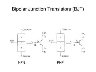
Bipolar Junction Transistors. Figure 5.5 Large-signal equivalent-circuit models of the npn BJT operating in the forward active mode. Figure 5.6 Cross-section of an npn BJT.


Bipolar Junction Transistors
E N D
Presentation Transcript
Figure 5.5 Large-signal equivalent-circuit models of the npn BJT operating in the forward active mode.
Figure 5.7 Model for the npn transistor when operated in the reverse active mode (i.e., with the CBJ forward biased and the EBJ reverse biased).
Figure 5.9 The iC –vCB characteristic of an npn transistor fed with a constant emitter current IE. The transistor enters the saturation mode of operation for vCB< –0.4 V, and the collector current diminishes.
Figure 5.10 Concentration profile of the minority carriers (electrons) in the base of an npn transistor operating in the saturation mode.
Figure 5.12 Large-signal model for the pnp transistor operating in the active mode.
Figure 5.14 Voltage polarities and current flow in transistors biased in the active mode.
Figure 5.16 The iC –vBE characteristic for an npn transistor.
Figure 5.17 Effect of temperature on the iC–vBE characteristic. At a constant emitter current (broken line), vBE changes by –2 mV/°C.
Figure 5.18 The iC–vCB characteristics of an npn transistor.
Figure 5.19 (a) Conceptual circuit for measuring the iC–vCE characteristics of the BJT. (b) The iC–vCE characteristics of a practical BJT.
Figure 5.20 Large-signal equivalent-circuit models of an npn BJT operating in the active mode in the common-emitter configuration.
Figure 5.21 Common-emitter characteristics. Note that the horizontal scale is expanded around the origin to show the saturation region in some detail.
Figure 5.22 Typical dependence of b on IC and on temperature in a modern integrated-circuit npn silicon transistor intended for operation around 1 mA.
Figure 5.23 An expanded view of the common-emitter characteristics in the saturation region.
Figure 5.24 (a) An npn transistor operated in saturation mode with a constant base current IB. (b) The iC–vCEcharacteristic curve corresponding to iB = IB. The curve can be approximated by a straight line of slope 1/RCEsat. (c) Equivalent-circuit representation of the saturated transistor. (d) A simplified equivalent-circuit model of the saturated transistor.
Figure 5.25 Plot of the normalized iC versus vCE for an npn transistor with bF = 100 and aR = 0.1. This is a plot of Eq. (5.47), which is derived using the Ebers-Moll model.
Figure 5.26 (a) Basic common-emitter amplifier circuit. (b) Transfer characteristic of the circuit in (a). The amplifier is biased at a point Q, and a small voltage signal vi is superimposed on the dc bias voltage VBE. The resulting output signal vo appears superimposed on the dc collector voltage VCE. The amplitude of vo is larger than that of vi by the voltage gain Av.
Figure 5.27 Circuit whose operation is to be analyzed graphically.
Figure 5.28 Graphical construction for the determination of the dc base current in the circuit of Fig. 5.27.
Figure 5.29 Graphical construction for determining the dc collector current IC and the collector-to-emitter voltage VCE in the circuit of Fig. 5.27.
Figure 5.30 Graphical determination of the signal components vbe, ib, ic, and vce when a signal component vi is superimposed on the dc voltage VBB (see Fig. 5.27).
Figure 5.31 Effect of bias-point location on allowable signal swing: Load-line A results in bias point QA with a corresponding VCEwhich is too close to VCCand thus limits the positive swing of vCE. At the other extreme, load-line B results in an operating point too close to the saturation region, thus limiting the negative swing of vCE.
Figure 5.32 A simple circuit used to illustrate the different modes of operation of the BJT.
Figure 5.43 Two obvious schemes for biasing the BJT: (a) by fixing VBE; (b) by fixing IB. Both result in wide variations in IC and hence in VCE and therefore are considered to be “bad.” Neither scheme is recommended.
Figure 5.44 Classical biasing for BJTs using a single power supply: (a) circuit; (b) circuit with the voltage divider supplying the base replaced with its Thévenin equivalent.
Figure 5.45 Biasing the BJT using two power supplies. Resistor RB is needed only if the signal is to be capacitively coupled to the base. Otherwise, the base can be connected directly to ground, or to a grounded signal source, resulting in almost total b-independence of the bias current.
Figure 5.46 (a) A common-emitter transistor amplifier biased by a feedback resistor RB. (b) Analysis of the circuit in (a).
Figure 5.47 (a) A BJT biased using a constant-current source I. (b) Circuit for implementing the current source I.
Figure 5.48 (a) Conceptual circuit to illustrate the operation of the transistor as an amplifier. (b) The circuit of (a) with the signal source vbe eliminated for dc (bias) analysis.
Figure 5.49 Linear operation of the transistor under the small-signal condition: A small signal vbe with a triangular waveform is superimposed on the dc voltage VBE. It gives rise to a collector signal current ic, also of triangular waveform, superimposed on the dc current IC. Here, ic = gmvbe, where gm is the slope of the iC–vBE curve at the bias point Q.
Figure 5.50 The amplifier circuit of Fig. 5.48(a) with the dc sources (VBE and VCC) eliminated (short circuited). Thus only the signal components are present. Note that this is a representation of the signal operation of the BJT and not an actual amplifier circuit.
Figure 5.51 Two slightly different versions of the simplified hybrid-p model for the small-signal operation of the BJT. The equivalent circuit in (a) represents the BJT as a voltage-controlled current source (a transconductance amplifier), and that in (b) represents the BJT as a current-controlled current source (a current amplifier).
Figure 5.52 Two slightly different versions of what is known as the T model of the BJT. The circuit in (a) is a voltage-controlled current source representation and that in (b) is a current-controlled current source representation. These models explicitly show the emitter resistance re rather than the base resistance rp featured in the hybrid-p model.
Figure 5.53 Example 5.14: (a) circuit; (b) dc analysis; (c) small-signal model.
Figure 5.55 Example 5.16: (a) circuit; (b) dc analysis; (c) small-signal model; (d) small-signal analysis performed directly on the circuit.
Figure 5.56 Distortion in output signal due to transistor cutoff. Note that it is assumed that no distortion due to the transistor nonlinear characteristics is occurring.
Figure 5.57 Input and output waveforms for the circuit of Fig. 5.55. Observe that this amplifier is noninverting, a property of the common-base configuration.