Transcriptome reconstruction and quantification
Transcriptome reconstruction and quantification. Outline. Lecture: algorithms & software solutions Exercises II: de-novo assembly using Trinity Exercises I: read-mapping and quantification using Cufflinks. The transcriptome ….

Transcriptome reconstruction and quantification
E N D
Presentation Transcript
Outline Lecture: algorithms & software solutions Exercises II: de-novo assembly using Trinity Exercises I: read-mapping and quantification using Cufflinks
The transcriptome… “… is everything that is transcribed in a certain sample under certain conditions” -> What sequences are transcribed? -> What are the transcripts? -> What are their expression patterns? -> What is their biological function? -> How are they transcribed and regulated? High-throughput sequencing: cost-efficient way to get reads from active transcripts.
RNA-Seq: a historic perspective • Traditional: sequence cDNA libraries by Sanger • Tens of thousands of pairs at most (20K genes in mammal) • Redundancy due to highly expressed genes • Not only coding genes are transcribed • Poor full-lengthness (read length about 800bp) • Indels are the dominant error mode in Sanger (frameshifts)
Next-Gen Sequencing technologies • 1 Lane of HiSeq yields 30GB in sequence • Error patterns are mostly substitutions • Good depth, high dynamic range • Full-length transcripts • Allow for expression quantification • Strand-specific libraries
The problem: • Reconstruct full-length transcripts (1000’s bp) from reads (100bp) • Read coverage highly variable • Capture alternative isoforms • Annotation? Expression differences? Novel non-coding? • Solution(?): • Read-to-reference alignments, assemble transcripts • (Cufflinks, Scripture) • Assemble transcripts directly (Trans-ABySS, Oases, Trinity)
Read mapping vs. de novo assembly Haas and Zody, Nature Biotechnology 28, 421–423 (2010)
Read mapping vs. de novo assembly Good reference No genome Haas and Zody, Nature Biotechnology 28, 421–423 (2010)
Transcriptome reconstruction with Cufflinks: How it works Cole Trapnell Adam Roberts Geo Pertea Brian Williams Ali Mortazavi Gordon Kwan Jeltjevan BarenSteven SalzbergBarbara Wold Lior Pachter
Workflow • Map reads to reference genome: • Disambiguate alignments • Allow for gaps (introns) • Use pairs (if available) • Build sequence consensus: • Identify exons & boundaries • Identify alternative isoforms • Quantify isoform expression • Differential expression: • Between isoforms (Expectation Maximization) • Between samples • Annotation-based and novel transcripts
Read-to-reference alignment Garber et al. Nature Methods 8, 469–477 (2011)
Read-to-reference alignment Garber et al. Nature Methods 8, 469–477 (2011)
Tophat Trapnell et al. Nature Biotechnology 28, 511–515 (2010)
Cufflinks Trapnell et al. Nature Biotechnology 28, 511–515 (2010)
Cufflinks Trapnell et al. Nature Biotechnology 28, 511–515 (2010)
Measure for expression: FPKM and RPKM • FPKM: Fragments Per Kilobase of exon per Million fragmentsmapped • RPKM: equivalent for unpaired reads • Longer transcripts, more fragments • FPKM/RPKM measure “average pair coverage” per transcript • Normalizes for total read counts • But it does NOT report absolute values (sum of transcripts constant)
Sensitivity and specificity as function of depth Trapnell et al. Nature Biotechnology 28, 511–515 (2010)
Alternative isoform quantification • Only reads that map to exclusive exons distinguish • Hundred reads might group many thousands • Robustness: Maximation Estimation (EM) algorithm
Comparative transcriptomics Kessmann et al. Nature 478, 343–348 (20 October 2011)
Transcriptome assembly with Trinity: How it works Brian Haas Moran Yassour Kerstin Lindblad-Toh Aviv Regev NirFriedman David Eccles AlexiePapanicolaou Michael Ott …
Workflow • Compress data (inchworm): • Cut reads into k-mers (k consecutive nucleotides) • Overlap and extend (greedy) • Report all sequences (“contigs”) • Build de Bruijn graph (chrysalis): • Collect all contigs that share k-1-mers • Build graph (disjoint “components”) • Map reads to components • Enumerate all consistent possibilities (butterfly): • Unwrap graph into linear sequences • Use reads and pairs to eliminate false sequences • Use dynamic programming to limit compute time (SNPs!!)
The de Bruijn Graph • Graph of overlapping sequences • Intended for cryptology • Minimum length element: k contiguous letters (“k-mers”) • CTTGGAA • TTGGAAC • TGGAACA • GGAACAA • GAACAAT
The de Bruijn Graph • Graph has “nodes” and “edges” • G GGCAATTGACTTTT… • CTTGGAACAAT TGAATT • A GAAGGGAGTTCCACT…
The de Bruijn Graph • Graph has “nodes” and “edges” • G GGCAATTGACTTTT… • CTTGGAACAAT TGAATT • A GAAGGGAGTTCCACT…
Iyer MK, Chinnaiyan AM (2011) Nature Biotechnology29, 599–600
Iyer MK, Chinnaiyan AM (2011) Nature Biotechnology29, 599–600
Iyer MK, Chinnaiyan AM (2011) Nature Biotechnology29, 599–600
Iyer MK, Chinnaiyan AM (2011) Nature Biotechnology29, 599–600
Inchworm Algorithm Decompose all reads into overlapping Kmers (25-mers) Identify seed kmer as most abundant Kmer, ignoring low-complexity kmers. Extend kmer at 3’ end, guided by coverage. G A GATTACA 9 T C
Inchworm Algorithm G 4 A GATTACA 9 T C
Inchworm Algorithm G 4 A 1 GATTACA 9 T C
Inchworm Algorithm G 4 A 1 GATTACA 9 T 0 C
Inchworm Algorithm G 4 A 1 GATTACA 9 T 0 C 4
Inchworm Algorithm G 4 A 1 GATTACA 9 T 0 C 4
Inchworm Algorithm G A 0 5 T 1 G C 4 0 A 1 GATTACA 9 T 0 G C 1 4 A 1 T C 1 1
Inchworm Algorithm G A 0 5 T 1 G C 4 0 A 1 GATTACA 9 T 0 G C 1 4 A 1 T C 1 1
Inchworm Algorithm A 5 G 4 GATTACA 9
Inchworm Algorithm A 5 C G 0 4 T 0 GATTACA A 9 6 G 1
Inchworm Algorithm A 5 G 4 GATTACA A 9 6 A 7 Report contig: ….AAGATTACAGA…. Remove assembled kmers from catalog, then repeat the entire process.
Inchworm Contigs from Alt-Spliced Transcripts=> Minimal lossless representation of data +
Chrysalis Integrate isoforms via k-1 overlaps
Chrysalis Integrate isoforms via k-1 overlaps
Chrysalis Integrate isoforms via k-1 overlaps Verify via “welds”
Chrysalis Integrate isoforms via k-1 overlaps Verify via “welds” Build de Bruijn Graphs (ideally, one per gene) Build de Bruijn Graphs (ideally, one per gene)
Result: linear sequences grouped in components, contigs and sequences >comp1017_c1_seq1_FPKM_all:30.089_FPKM_rel:30.089_len:403_path:[5739,5784,5857,5863,353] TTGGGAGCCTGCCCAGGTTTTTGCTGGTACCAGGCTAAGTAGCTGCTAACACTCTGACTGGCCCGGCAGGTGATGGTGAC TTTTTCCTCCTGAGACAAGGAGAGGGAGGCTGGAGACTGTGTCATCACGATTTCTCCGGTGATATCTGGGAGCCAGAGTA ACAGAAGGCAGAGAAGGCGAGCTGGGGCTTCCATGGCTCACTCTGTGTCCTAACTGAGGCAGATCTCCCCCAGAGCACTG ACCCAGCACTGATATGGGCTCTGGAGAGAAGAGTTTGCTAGGAGGAACATGCAAAGCAGCTGGGGAGGGGCATCTGGGCT TTCAGTTGCAGAGACCATTCACCTCCTCTTCTCTGCACTTGAGCAACCCATCCCCAGGTGGTCATGTCAGAAGACGCCTG GAG >comp1017_c1_seq2_FPKM_all:4.913_FPKM_rel:2.616_len:525_path:[2317,2791] CTGGAGATGGTTGGAACAAATAGCCGGCTGGCTGGGCATCATTCCCTGCAGAAGGAAGCACACAGAATGGTCGTTAAGTA ACAGGGAAGTTCTCCACTTGGGTGTACTGTTTGTGGGCAACCCCAGGGCCCGGAAAGGACAGACAGAGCAGCTTATTCTG TGTGGCAATGAGGGAGGCCAAGAAACAGATTTATAATCTCCACAATCTTGAGTTTCTCTCGAGTTCCCACGTCTTAACAA AGTTTTTGTTTCAATCTTTGCAGCCATTTAAAGGACTTTTTGCTCTTCTGACCTCACCTTACTGCCTCCTGCAGTAAACA CAAGTGTTTCAGGCAAAGAAACAAAGGCCATTTCATCTGACCGCCCTCAGGATTTAGAATTAAGACTAGGTCTTGGACCC CTTTACACAGATCATTTCCCCCATGCCTCTCCCAGAACTGTGCAGTGGTGGCAGGCCGCCTCTTCTTTCCTGGGGTTTCT TTGAATGTATCAGGGCCCGCCCCACCCCATAATGTGGTTCTAAAC >comp1017_c1_seq3_FPKM_all:3.322_FPKM_rel:2.91_len:2924_path:[2317,2842,2863,1856,1835] CTGGAGATGGTTGGAACAAATAGCCGGCTGGCTGGGCATCATTCCCTGCAGAAGGAAGCACACAGAATGGTCGTTAAGTA ACAGGGAAGTTCTCCACTTGGGTGTACTGTTTGTGGGCAACCCCAGGGCCCGGAAAGGACAGACAGAGCAGCTTATTCTG TGTGGCAATGAGGGAGGCCAAGAAACAGATTTATAATCTCCACAATCTTGAGTTTCTCTCGAGTTCCCACGTCTTAACAA AGTTTTTGTTTCAATCTTTGCAGCCATTTAAAGGACTTTTTGCTCTTCTGACCTCACCTTACTGCCTCCTGCAGTAAACA