Analysis Tools
Analysis Tools. What is an Algorithm?. An algorithm is a finite set of instructions that specify a sequence of operations to be carried out in order to solve a specific problem or class of problems. Algorithm Properties. An algorithm must possess the following properties:


Analysis Tools
E N D
Presentation Transcript
What is an Algorithm? An algorithm is a finite set of instructions that specify a sequence of operations to be carried out in order to solve a specific problem or class of problems.
Algorithm Properties An algorithm must possess the following properties: • Finiteness: Algorithm must complete after a finite number of instructions have been executed. • Absence of ambiguity: Each step must be clearly defined, having only one interpretation. • Definition of sequence: Each step must have a unique defined preceding & succeeding step. The first step (start step) & last step (halt step) must be clearly noted. • Input/output: There must be a specified number of input values, and one or more result values. • Feasibility: It must be possible to perform each instruction.
Analyzing an Algorithm In order to learn more about an algorithm, we can analyze it. That is, draw conclusions about how the implementation of that algorithm will perform in general. This can be done in various ways. • determine the running time of a program as a function of its inputs; • determine the total or maximum memory space needed for program data; • determine the total size of the program code; • determine whether the program correctly computes the desired result; • determine the complexity of the program--e.g., how easy is it to read, understand, and modify; and, • determine the robustness of the program--e.g., how well does it deal with unexpected or erroneous inputs?
Analyzing an Algorithm Different ways of analyzing the algorithm with render different results. An algorithm that runs fast is not necessarily robust or correct. An algorithm that has very little lines of code does not necessarily use less resources. So, how can we measure the efficiency of an algorithm?
Design Considerations Given a particular problem, there are typically a number of different algorithms that will solve that problem. A designer must make a rational choice among those algorithms: • To design an algorithm that is easy to understand, implement, and debug (software engineering). • To design an algorithm that makes efficient use of the available computational resources (data structures and algorithm analysis)
Example Replaced by Gauss summation sum N(N+1)/2 More efficient, but need to be as smart as 10-year-old Gauss. Easy to understand, but slow. Gauss Summation: http://www.cut-the-knot.org/Curriculum/Algebra/GaussSummation.shtml
Algorithm Analysis in CSCI 3333 But, how do we measure the efficiency of an algorithm? Note that the number of operations to be performed and the space required will depend on the number of input values that must be processed.
Benchmarking algorithms It is tempting to measure the efficiency of an algorithm by producing an implementation and then performing benchmarking analysis by running the program on input data of varying sizes and measuring the “wall clock” time for execution. However, there are many factors that affect the running time of a program. Among these are the algorithm itself, the input data, and the computer system used to run the program. The performance of a computer is determined by • the hardware: • processor used (type and speed), • memory available (cache and RAM), and • disk available; • the programming language in which the algorithm is specified; • the language compiler/interpreter used; • the computer operating system software.
Asymptotic Analysis Therefore, the goal is to have a way of describing the inherent complexity of a program, independent of machine/compiler considerations. This means not describing the complexity by the absolute time or storage needed. Instead, focus should be concentrated on a "proportionality" approach, expressing the complexity in terms of its relationship to some known function and the way the program scales as the input gets larger. This type of analysis is known as asymptotic analysis.
Asymptotic Analysis There is no generally accepted set of rules for algorithm analysis. In some cases, an exact count of operations is desired; in other cases, a general approximation is sufficient. Therefore, we strive to setup a set of rules to determine how operations are to be counted.
Analysis Rules To do asymptotic analysis, start by counting the primitive operations in an algorithm and adding them up. Assume that primitive operations will take a constant amount of time, such as: • Assigning a value to a variable • Calling a function • Performing an arithmetic operation • Comparing two numbers • Indexing into an array • Returning from a function • Following a pointer reference
Example of Counting Primitive Operations Inspect the pseudocode to count the primitive operations as a function of the input size (n) • Algorithm arrayMax(A,n): • currentMax ¬ A[0] • for i ¬ 1 to n – 1 do • if currentMax < A[i] then • currentMax ¬ A[i] • return currentMax • Count • Array indexing + Assignment 2 • Initializing i 1 • Verifying i<n n • Array indexing + Comparing 2(n-1) • Array indexing + Assignment 2(n-1) worst • Incrementing the counter 2(n-1) • Returning 1 Best case: 2+1+n+4(n–1)+1 = 5n Worst case: 2+1+n+6(n–1)+1 = 7n-2
Best, Worst, or Average Case Analysis An algorithm may run faster on some input data than on others. Best case – the data is distributed so that the algorithm runs fastest Worst case – the data distribution causes the slowest running time Average case – very difficult to calculate For our purposes, will concentrate on analyzing algorithms by identifying the running time for the worst case data.
Estimating the Running Time The actual running time depends on the speed of the primitive operations—some of them are faster than others • Let t = speed of the slowest primitive operation = worst case scenario • Let f(n) = the worst-case running time of arrayMax f(n) = t (7n – 2)
Growth Rate of a Linear Loop Growth rate of arrayMax is linear. Changing the hardware alters the value of t, so that arrayMax will run faster on a faster computer. However, growth rate is still linear. Slow PC 10(7n-2) Fast PC 5(7n-2) Fastest PC 1(7n-2)
Growth Rate of a Linear Loop What about the following loop? for (i=0; i<n; i+=2 ) do something Here, the number of iterations is half of n. However, higher the factor, higher the number of loops. So, although f(n) = n/2, if you were to plot the loop, you would still get a straight line. Therefore, this is still a linear growth rate.
Growth Rate of a Logarithmic Loop What about the following segments? for (i=1; i<n; i*=2 ) for (i=n; i>=1; i/=2 ) do something do something When n=1000, the loop will iterate only 10 times. It can be seen that the number of iterations is a function of the multiplier or divisor. This kind of function is said to have logarithmic growth, where f(n) = log n
Growth Rate of a Linear Logarithmic Loop What about the following segments? for (i=1; i<n; i++ ) for (j=1; j<n; j*=2 ) do something Here, the outer loop has a linear growth, and the inner loop has a logarithmic growth. Therefore: f(n) = n log n
Growth Rates ofCommon Classes of Functions Exponentially Quadratically Linearly Logarithmically Constant
Is This Really Necessary? Is it really important to find out the exact number of primitive operations performed by an algorithm? Will the calculations change if we miss out one primitive operation? In general, each step of pseudo-code or statement corresponds to a small number of primitive operations that does not depend on the input size. Thus, it is possible to perform a simplified analysis that estimates the number of primitive operations, by looking at the “big picture”.
What exactly is Big-O? • Big-O expresses an upper bound on the growth rate of a function, for sufficiently large values of n. • Upper bound is not the worst case. What is being bounded is not the running time (which can be determined by a given value of n), but rather the growth rate for the running time (which can only be determined over the range of values for n).
Big-Oh Notation Definition: Let f(n) and g(n) be functions mapping nonnegative integers to real numbers. Then, f(n) is O(g(n)) ( f(n) is big-oh of g(n) ) if there is a real constant c>0 and an integer constant n0³1, such that f(n) £cg(n) for every integer n³n0 By the definition above, demonstrating that a function f is big-O of a function g requires that we find specific constants C and N for which the inequality holds (and show that the inequality does, in fact, hold).
Big-O Theorems For all the following theorems, assume that f(n) is a function of n and that K is an arbitrary constant. • Theorem1: K is O(1) • Theorem 2: A polynomial is O(the term containing the highest power of n) f(n) = 7n4 + 3n2 + 5n + 1000 is O(7n4) • Theorem 3: K*f(n) is O(f(n)) [that is, constant coefficients can be dropped] g(n) = 7n4 is O(n4) • Theorem 4: If f(n) is O(g(n)) and g(n) is O(h(n)) the f(n) is O(h(n)). [transitivity]
Big-O Theorems • Theorem 5: Each of the following functions is strictly big-O of its successors: K [constant] logb(n) [always log base 2 if no base is shown] n nlogb(n) n2 n to higher powers 2n 3n larger constants to the n-th power n! [n factorial] nn For Example: f(n) = 3nlog(n) is O(nlog(n)) and O(n2) and O(2n) smaller larger
Big-O Theorems • Theorem 6: In general, f(n) is big-O of the dominant term of f(n), where “dominant” may usually be determined from Theorem 5. f(n) = 7n2+3nlog(n)+5n+1000 is O(n2) g(n) = 7n4+3n+106 is O(3n) h(n) = 7n(n+log(n)) is O(n2) • Theorem 7: For any base b, logb(n) is O(log(n)).
Examples In general, in Big-Oh analysis, we focus on the “big picture,” that is, the operations that affect the running time the most – the loops Simplify the count: • Drop all lower-order terms 7n – 2 7n • Eliminate constants 7n n • Remaining term is the Big-Oh 7n – 2 is O(n)
More Examples Example: f(n) = 5n3 – 2n2 + 1 • Drop all lower order terms 5n3 – 2n2 + 1 5n3 • Eliminate the constants 5n3 n3 • The remaining term is the Big-Oh f(n) is O(n3)
Determining Complexities in General • We can drop the constants • sum rule: for a sequential loops add their Big-Oh values statement 1; statement 2; ... statement k; total time = time(statement 1) + time(statement 2) + ... + time(statement k) • if-then-else statements: the worst-case time is the slowest of the two possibilities if (cond) { sequence of statements 1 } else { sequence of statements 2 } Total time = max(time(sequence 1), time(sequence 2))
Determining Complexities in General • for loops: The loop executes N times, so the sequence of statements also executes N times. Since we assume the statements are O(1), total time = N * O(1) = O(N) • Nested for loops: multiply their Big-Oh values for (i = 0; i < N; i++) { for (j = 0; j < M; j++) { sequence of statements } } total time = O(N) * O(M) = O(N*M) • In a polynomial, the term with the highest degree establishes the Big-Oh
Why Does Growth Rate Matter? Assuming that it takes 0.4 nsec to process one element
Finding the Big-Oh for( int i=0; i<n; ++i ) { for(int j=0; j<n; ++j) { myArray[i][j] = 0; } } sum = 0; for( int i=0; i<n; ++i ) { for(int j=0; j<i; ++j) { sum++; } }
Example that shows why the Big-Oh is so important. Write a program segment so that, given an array X, compute array A such that, each number A[i] is the average of the numbers in X from X[0] to X[i] X 1 3 5 7 9 X[0] + X[1] + X[2] = 9 9 / 3 = 3 1 2 3 4 5 A
Solution #1 – Quadratic time • Algorithm prefixAverages1 … for i ¬ 0 to n-1 do a ¬ 0 for j ¬ 0 to i do a ¬ a + X[j] A[i] ¬ a/(i+1) … • Two nested loops Inner loop – loops through X, adding the numbers from element 0 through element i Outer loop – loops through A, calculating the averages and putting the result into A[i]
Solution #2 - Linear Time • Algorithm prefixAverages2 … s ¬ 0 for i ¬ 0 to n-1 do s ¬ s + X[i] A[i] ¬ s/(i+1) … • Only one loop Sum – keeps track of the sum of the numbers in X so that we don’t have to loop through X every time Loop – loops through A, adding to the sum, calculating the averages, and putting the result into A[i]
Lessons Learned • Both algorithms correctly solved the problem • Lesson – There may be more than one way to write your program. • One of the algorithms was significantly faster • Lesson – The algorithm that we choose can have a big influence on the program’s speed. Evaluate the solution that you pick, and ask whether it is the most efficient way to do it.