Download
1 / 18
180 likes | 283 Vues
Explore particle methods for rarefied gas and two-phase flows, examining Boltzmann equation, scales of the problem, Lagrangian and Eulerian approaches, and effects of particle-fluid interactions.

E N D
Some issues and methods inparticles tracking Laurent DUMAS Université Paris 6 (L.AN.) & Ecole Normale supérieure (D.M.I.) • Lecture 1 (August 19th): an academical survey • Particle methods for rarefied gas and two phase flows • Lecture 2 (August 27th): an industrial approach • Slag deposition and pressure oscillations in Ariane V boosters
Particle methods for rarefied gas and two phase flows 1. Introduction 2. The Boltzmann equation 3. Scales of the problem 4. The Lagrangian approach 4.1 Construction of particle methods 4.2 Examples of simulations 5. The Eulerian approach 6. Effects on particles of the fluid turbulence 6.1 RANS simulations 6.2 LES simulations 7. Effects of particles on the fluid turbulence 8. Justification of particle self diffusion in a simple case
1. Introduction • Rarefied flows are encountered in space and nuclear engineering • Two phase flows (liquid or solid droplets in a gas) appears in meteorology (particulate pollution), car propulsion, electrical power generation (vaporization of liquid droplets of fuel), etc…. • Two phase flows can be classified as being either dilute, semi-dilute or dense . Only in the first case, the particles are supposed to be independent (no collision process). • An exact model is far beyond computational capabilities • The particle tracking can be achieved in a one way or two waycoupling, by using a Lagrangian or a Eulerian approach.
2. The Boltzmann equation • f(t,x,r,v): probability distribution function of particles of radius r, at position x, time tand with velocity v: • plus initial and boundary conditions. • b: acceleration of a particle • w: evaporation rate (dropped from now on) • Q(f ): collision effects
The particle acceleration • For two phase flows, is given by the Odar Hamilton equation: • I: external field (gravity) • II: generalizedArchimede force (dropped from now on) • III: drag force • IV: jet propulsion effect (dropped from now on)
The drag force • The drag force is approximated by the expression: • with:
The collision kernel with (elastic collisions and hard spheres model) r v-v1 n r1
3. Scales of the problem • Time scales: • c: mean free time between two collisions. • : smallest time scale of the flow ( ). • p (two phase flow): particle characteristic time ( p=rpd2/18m ). • l: turbulence time scale ( ) • T: macroscopic characteristic time • Length scale: • d: diameter of a particle. • Characteristic numbers: • Re, Re p: Reynolds numbers (Re=rpUL/m). • Kn: Knudsen number (Kn= c / T). • St (two phase flow): Stokes number (St= p / T). • ap: particle volumetric fraction (ap = Nm / Vr)
4. The Lagrangian approach:general algorithm of particle methods The idea is to seek a solution of the Boltzmann equation of the form: and to split the convective and the collision part. Algorithm • 1. Generate N particles using the initial PDF • 2. Integrate the ordinary differential equation on a small time interval for each particle • 3. In each cell, make the appropriate number of collisions between random particles.
Collision process in the homogeneous case The previous solution f of the homogeneous Boltzmann equation satisfies for each test function : The time step is chosen such that and the collision process is then achieved in the following way: • 1 For each pair of particle, choose s randomly in [0,1]. • 2. If , make a collision and choose the outgoing velocities (or and ) with the law
5. The Eulerian approach • Take the first moments of the Boltzmann equation and get: • mass conservation: • momentum conservation: • with p: particle volumetric fraction • , • p: mean particle relaxation time
6.1 Effects on particles of the fluid turbulencewith RANS models (Case 1: Lagrangian approach) • Hypothesis: no interactions between particles • ug is replaced during a time t by <ug>+u’ where u’ is selected from a Gaussian distribution with a variance related to the turbulence energy (2k/3). t is deduced from the lifetime of the energy containing eddy and allows for the particle to pass through the eddy before it decayed (Gossman, Ioannides, 1981). • Many variants: Berlemont (1990), Zhou and Leschnizer (1991),...
A theoretical result on a Gossmann Ioannides type model Theorem (J.F. Clouet, K. Domelevo, 1997): assume that the acceleration is given by: and that the decorrelation time t, k and ug are constants. Then the expectation F of all the realizations of the corresponding random Boltzmann equation is solution of the equation where Dx(t) and Dv (t) and given by explicit formulas.
6.1 Effects on particles of the fluid turbulencewith RANS models (Case 2: Eulerian approach) • The mass conservation equation is now: • where the dispersion coefficient D is semi-empirically determined. • In the momentum conservation equation, a Reynolds-stress like tensor appears and is usually modelized using the Boussinesq approximation.
6.2 Effects on particles of the fluid turbulencewith LES models • Case 1 (the Lagrangian approach): • During a time step (equal to the one used for the fluid velocity calculation), each particle is displaced solving the equation of movement with • The detection of eventual collisions during this process can also be implemented. Moreover, the interaction with the gas flow leads to correlate the velocities of neighboring particles. • Case 2 (the Eulerian approach): • As in the case of RANS models, an assumption is made to modelise the Reynolds-stress like tensor appearing in the particle momentum equation.
7. Effects of particles on the fluid turbulence • Some experimental or numerical data show that small particles will attenuate turbulence while large particles will generate it. • To include the effects of particles (two-way coupling), the usual approach is to modify the fluid equations for turbulence and dissipation (in RANS simulations) or the subgrid scale model (in LES simulations). A force term can also be added in the gas momentum equation. • See a review by Crowe, Troutt, Chung (Ann. Rev. Fl. Mech., 1996)
Diagram of turbulence modulation p/ l Particles enhance turbulence 1 Negligible effects on turbulence Particles decay turbulence ap 10-6 10-3 One way coupling Two way coupling dilute suspension dense suspension
8. Justification of the particle self diffusion in a simple case • Consider a set of colliding particles suspended in homogeneous and stationnary gas turbulence. It is numerically observed (with LES simulations for instance) that the quantity • tends to a constant value for long time dispersion (particle self diffusion): • Some approximate values of D have been proposed (Simonin). In particular, when c « p and l « p (collisions are predominant), it is • found that Dcq2