Management Plan
Management Plan. User Plane. Control Plane. Applications. Signaling Protocol. Native. TCP/IP. AAL. ATM Layer. Physical Layer. B-ISDN Protocol Reference Model. SNMP: Simple Network Management Protocol CMIP: Common Management Information Protocol. Control Plane

Management Plan
E N D
Presentation Transcript
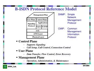
Management Plan User Plane Control Plane Applications Signaling Protocol Native TCP/IP AAL ATM Layer Physical Layer B-ISDN Protocol Reference Model SNMP: Simple Network Management Protocol CMIP: Common Management Information Protocol • Control Plane • Supports Signaling • Call Setup, Call Control, Connection Control • User Plane • Data Transfer, Flow Control, Error Recovery • Management Plane • Operation, Administration, & Maintenance
Management Plane (Provides control of ATM switch) Layer Management (Layered) Plane Management (No Layered) • Concerned with management of all the planes • All management functions (Fault, Performance, Configuration, Operation, & Security) which relates to the whole system are located in the Plane Management • Provides coordination between all planes • Use to manage each of the ATM layers with entity corresponding to each ATM layer • OAM issues
VideoImageDataetc… USER USER ATM SW ATM SW USER USER NNI UNI UNI Higher Layers Higher Layers • Flow Control • Error Handling • Message Segmentation ConvergenceSublayers (CS) ConvergenceSublayers (CS) AdaptationLayer • Segmentation Type • Message Number • Message ID SegmentationReassemblySublayer (SAR) SegmentationReassemblySublayer (SAR) • 5 Byte Header • 48 Byte Payload • Handles cont. and bursty traffic ATM Layer ATM Layer ATM Layer ATM Layer • SONET USER USER Physical Layer Physical Layer Physical Layer Physical Layer Broadband Networking with SONET and ATM
ATM Protocol Reference Model in the User Plane Upper Layers Abbreviations AAL = ATM Adaptation Layer SAR = Segmentation and Reassembly CS = Convergence Sublayer PL = Physical Layer TC = Transmission Convergence PM = Physical Medium class A class B class C class D 1 2 3 4 • Handling lost / misdelivered cells • Timing recovery • Interleaving CellInformationField CS AAL • Split frames / bit stream info cells • Re-assemble frames / bit stream SAR Service Classes for AAL Class Type • Cell routing • Multiplexing / demultiplexing • Generic flow control CellHeader Constant Bit Rate Variable Bit Rate Connection Oriented Data Connectionless Data A B C D ATM • Cell header verification and cell delineation • Rate decoupling (insert idle cells) • Transmission frame adaptation TC PL • SEAL = Simple and Efficient Adaptation Layer • Type 5 AAL • Acknowledged info transfer • Bit timing • Physical medium PM Remark: See next page
Remarks: PMD Physical Medium Dependent TC Transmission Convergence Sublayer It separates transmission from the physical interface and allows ATM interfaces to be built on a large variety of physical interfaces
a) Physical Medium (PM) PM sublayer provides the bit transmission capability including bit alignment Line coding and, if necessary, electrical/optical conversion is performed in this sublayer Optical fiber is used for the physical medium. Other media, coax cables are also possible Bit rates 155 Mbps or 622.080 Mbps. Physical Layer Functions
b) Bit Timing Generation and reception of waveforms which are suitable for the medium, the insertion, and extraction of bit timing information and the line coding if required CMI (Code Mark Inversion) (CCITT G.703) proposed for 155.520 Mbps interface. NRZ “Nonreturn to Zero” code proposed for optical interface. Physical Layer Functions
Electrical Interface:Coded Mark Inversion (CMI) For binary 0 always a positive transition at the midpoint of the binary unit time interval. For binary 1 always a constant signal level for the duration of the bit time. This level alternates between high and low for successive binary 1s. Line Coding 0 1 0 0 1 1 0 0 0 1 1 Level A2 Level A1
Optical Interface:Nonreturn to Zero (NRZ) For binary 0 Emission of light For binary 1 No emission of light Transition: 0 1 or 1 0Otherwise no transition Line Coding (cont.) 0 1 0 0 1 1 0 0 0 1 1 Level A2 Level A1
ATM INTERFACES • SONET/SDH : 155 Mbps and 622 Mbps over OC-3 (single mode fiber) • Cell Based • PDH Based (ATM cells mapped into PDH signals) • (59 columns and 9 rows • frame). Frame at 34.368 Mbps. • FDDI based or 100 Mbps (same as in FDDI PMD uses multimode fiber and • line coding of 4B/5B). (called TAXI interface). Early private UNI interfaces • were based on TAXI interfaces. • DS-3 (45 Mbps) Transfer of ATM cells on T3 (DS-3) public carrier interface. • It is cheaper than SONET links. • STS-3 (155 Mbps) over Multimode fiber uses line coding of 8B/10B. • STS-3 (155 Mbps) over Twisted Pair (using Taxi interface) uses line coding • of 8B/10B. • D1-T1 carriers (1.5 Mbps) IFA’2004
CELL BASED INTERFACE • This interface consists of a continuous stream of cells where • each cell contains 53 octets. 26 26 0 1 0 1 Physical layer OAM cell • Synchronization achieved through HEC basis. • Maximum spacing between successive physical layer cells is • 26 ATM layer cells. • After 26 consecutive ATM layer cells, a physical layer cell (idle • cells or OAM cells) is enforced to adapt transfer capability to • the interface rate. IFA’2004
Transmission Convergence Sublayer (TC) • Transmission Frame Adaptation • Adapts the cell flow according to the used payload structure of the transmission system in the sending direction. • In the opposite direction, it extracts the cell flow out of the transmission frame. IFA’2004
2. Header Error Control (HEC) • After initialization receiver is in the “Correction Mode” • Single bit error detected corrected • Multiple bit error detected cell discarded • Receiver switches to “Detection Mode” • In “Detection Mode”, each cell with a detected single-bit error is discarded. • If a correct header is found, receiver switches to • “Correction Mode” Multiple-bit errror (Cell discarded) Error detectedCell discarded NoError Correction Mode No error Detection Mode Correction Single-bit error IFA’2004
Example: p Probability that a bit is in error (1-p) Probability that a bit is NOT in error p40 Probability that 40 bits are in error (1-p)40 Probability that 40 bits are correct
a) With what probability a cell is rejected when the HEC state machine is in the "Correction Mode"? Correction Mode Probability of a cell being rejected Different Perspective: When is a cell accepted? * Probability of having no errors in cell header OR * Probability of having a single bit error in cell header
With what probability a cell is rejected when the HEC state machine is in the "Detection Mode"? Detection Mode HEC will only accept ERROR-FREE cells. Different Perspective: What is the probability that a cell header is correct?
Assume that the HEC state machine is in the “Correction Mode.” What is the probability that n successive cells will be rejected, where n >= 1 ? Correction Mode Probability of n successive cells being accepted (n>1) n=1: Probability that 1 cell is accepted, i.e., the entire header is error-free. What is that probability? OR There is at most one bit error in the header. What is that probability?
1 2 n=2: Probability that the cell header (2) is correctAND Previous case for cell 1 OR Probability that the cell header (2) has at most 1 bit errorAND Probability that the cell header (1) is correct (error free)
3 1 2 n=3: Probability that the cell header (3) is correctAND Previous case for cell n=1 OR Probability that the cell header (3) has at most 1 bit errorAND Probability that the cell header (2) is correctANDThe case for n=1
Assume that the HEC state machine is in the “Correction Mode.” What is the probability p(n) that n successive cells will be accepted, where n >= 1 ? First cell is rejected: What is the probability that a cell is rejected? Case a) Different Perspective: Probability that all header bits of a cell are correct Probability that one single bit error in a cell header
Remaining n-1 successive cells: Now, HEC is in Detection Mode What is the probability that (n-1) successive cells are rejected, i.e., there will be errors in the headers for the remaining (n-1) cells
EFFECT OF ERROR IN CELL HEADER Incoming Cell Error in Header? No Valid cell (intended service) Yes Apparently valid cell With errored header (unintended service) Error detected No Yes Current mode? Detection Discarded Cell Correction Error incorrectable? Yes No Correction attempt Unsuccessful Successful IFA’2004
Every ATM cell transmitter calculates the HEC value across the first 4 octets of the cell header and inserts the result in the fifth octet (HEC field) of the cell header. The HEC value is defined as “the remainder of the division (modulo 2) by the generator polynomial x8+x2+x+1 of the product x8 multiplied by the content of the header excluding the HEC field to which the fixed pattern 01010101 will be added modulo 2.” The receiver must subtract first the coset value of the 8 HEC bits before calculating the syndrome of the header. Device always preset to 0s. [Key Word: CRC (Cyclic Redundancy Check Algorithm)] HEC Generation Algorithm (I.432)
ATM CELL STRUCTURE 8 7 6 5 4 3 2 1 Octet 1 2 3 4 5 : : : 53 HEADER (5 octets) PAYLOAD (48 octets) 8 7 6 5 4 3 2 1 1 2 3 4 5 : : 53 GFC VPI VPI VCI VCI VCI PT PR HEC PAYLOAD (48 octets)
The HEC field contains the 8-bit FCS (Frame Check Sequence) obtained by dividing the first 4 octets (32 bits) of the cell header multiplied by 2^8 by the CRC code (generator polynomial) (x8+x2+x+1) HEC Generation Algorithm
This HEC code can Correct single bit errors Detect multiple bit errors HEC Generation Algorithm (I.432) Purpose: • Protects the header control information • Helps to find a valid cell (cell delineation and boundaries)
CELLDELINEATION (This process allows identification of cell boundaries) Correct HEC Bit-by-Bit Cell-by-Cell HUNT PRESYNC Incorrect HEC consecutive incorrect HEC consecutive correct HEC SYNCH
In Hunt State a cell delineation algorithm is performed bit-by-bit to determine if the HEC coding law is observed (i.e., match between received HEC and calculated HEC). Once a match is achieved, it is assumed that one header has been found and the method enters the PRESYNCH state. The HEC algorithm is performed cell-by-cell. If consecutive correct HECs are found, SYNCH state is entered; if not the system goes back to HUNT state. SYNCH is only left (to HUNT) state if consecutive incorrect HECs are identified. Cell Delineation (cont.)
and are design parameters that influence the performance of cell delineation process.(=7 and =6). Greater values of result in longer delays in recognizing a misalignment but in a greater robustness against false alignment. Greater values of result in longer delays in establishing synchronization but in greater robustness against false delineation. Cell Delineation (cont.)
Cell Delineation (cont.) • Remarks: • A 155.520 Mbps ATM system will be in SYNCH state for more than 5349 years even when the bit error probability is BER=10-4. • This method may fail if the header HEC occurs in the info field (maliciously or accidentally) Cell Payload Scrambling. • To overcome the info field contents scrambled using a self-synchronizing scrambler with polynomial X43 + 1. Header itself is not scrambled.
The probability of 7 consecutive incorrect HEC withBER=10-4 A= The probability that 7 consecutive cells are in error.[1- (1-10-4)40 ]7 = 1.616*10-17 = A 1/A The number of cells sent in order to have a 7 consecutive error cells; (Unit Cells);How often does event A occur in terms of ATM cells.
{53 * 8} / {155.52 Mbps} = C (53*8) = # of bits/cell ; Link Speed = # of bits/sec How long does it take to send one ATM cell through the 155 Mbps link.{[1 / { A}] * C ={6.187*106} * 53 * 8} / {155.52 Mbps} = 1.6868*1011 = 5349 Years End Result in terms of seconds End result/(365*24*60*60) approx. 5349 years..
Cell Rate Decoupling (Speed Matching) • Adapts cell stream into Transmission Bit Rate (Insertion / Discarding idle cells; in particular for SONET Interface). SONET uses synchronous cell time slots! • Note: Cell Based Interface No need for this function.
ATM Transmitter ATM Receiver VPI/VCI VPI/VCI B u f f e r + - VPI/VCI Remove the Idle or Unassigned cells Insert Idle or Unassigned cells Cell Rate Decoupling (cont.) (Speed Matching) Transmitter multiplexes multiple streams; queueing them if an ATM cell is not immediately available. If the queue is empty, when the time arrives to fill the next synchronous cell time slot, then the Transmission Convergence Sublayer inserts an Idle cell (or the ATM layer inserts an Unassigned cell.)
ATM Layer Functions • Cell Multiplexing/Demultiplexing • Cell VPI/VCI Translation • Cell Header Generation/Extraction • GFC Function
ATM Layer Functions (Cont’d) • Cell Multiplexing/Demultiplexing • In the transmit direction, cells from individual VPs and VCs are multiplexed into one resulting stream. • At the receiving side the cell demultiplexing function splits the arriving cell stream into the individual cell flows appropriate to the VP or VC.
ATM Layer Functions (cont.) ii)Cell VPI/VCI Translation - At ATM switching nodes, the VPI and VCI translation must be performed. - Within VP switch, the value of the VPI field of each incoming cell is translated into a new VPI value for the outgoing cell. - At a VC switch, the values of the VPI as well as the VCI are translated into new values.
ATM Layer Functions (cont.) iii)Cell Header Generation / Extraction - This function is applied at the termination points of the ATM layer. - Transmit Side: After receiving the cell information from the AAL, the cell header generation adds the appropriate ATM cell header except for the HEC values. HEC is done at Physical Layer. VPI/VCI values could be obtained by a translation from the SAP identifier. - Receive Side: The cell header extraction function removes the cell header. Only the cell information is passed to the AAL. - This function could also translate a VPI/VCI value into a SAP identifier.
ATM Layer Functions (cont.) iv)GFC functions - Supports the control of the ATM traffic flow in a UNI. It can be used to alleviate short overload conditions. - Control of cell flows toward the network but not flow control from the network. - No effect within the network.
Virtual Path and Virtual Circuit Concept • ATM cells flow along entities known as VIRTUAL CHANNELS. A VC is identified by its virtual circuit identifier (VCI). • VC set up between 2 end-users (like VC in X.25 => Indiv. Log connection). • VP Bundle of VCs having the same end points (Group logical connection; reserved trunk of connections). • All cells in a given VC follow the same route across the network and are delivered in the order they were transmitted. • VCs are transported within Virtual Paths (VPs). A VP is identified by its virtual path identifier (VPI). VPs are used for aggregating VCs together or for providing an unstructured data pipe.
Virtual Path and Virtual Circuit Concept • Optical links will be capable of transporting hundreds of Mbps where VCs fill kbps. Thus, a large number of simultaneous channels have to be supported in a transmission link. Typically 10K simultaneous channels are considered (thus, VCI field up to 16bits). • Since ATM is connection oriented, each connection is characterized by a VCI which is assigned at Call-Set-Up. • When connection is released, VCI values on the involved links will be released or can be reused by other components.
VIRTUAL PATH / VIRTUAL CIRCUIT CONCEPT VP TRANSMISSIONPATH VC Virtual Path Text VCI =1 (text) Voice VCI =2 (voice) Video VCI =3 (video) ATM Network Interface
VIRTUAL PATH/VIRTUAL CIRCUIT CONCEPT • Each VP has a different VPI value and each VC within a VP has a different value. • Two VCs belonging to different VPs at the same interface may have identical VCI values. • VPI is changed at points where a VP link is terminated. • VCI is changed at points where a VC link is terminated.
Goal Multimedia Communication • Video & Voice Time Sensitive (Delay bounds) • Data Loss Sensitive (Loss bounds) • Allows the network to add or remove components during the connection e.g. Video Telephony Start with voice (only single VC) Add video later (on another VC) Add data (on another VC) Signaling (on another VC)
EXAMPLE • Three VP connections exist from A to B. They are seen by A as corresponding to the values p, q, r of the VPI field, and by B as corresponding to the values p2, q2, r2. Whenever A wants to send some information to B on the VP connection seen as p, it writes the value p in the VPI field of the cell. • The VP switches T1, T2 and T3 swap the VPI labels according to the lookup tables. The VCI field is not changed by the VP switches, so it can be used by A to multiplex several VC connections on any one of the three VP connections. Therefore, at the VC level, A has at its disposal three direct links to B. A VP Level B A VC Level B p p2 p p2 p1 T1 T2 q q2 q q2 T3 r r2 r r2
VCI 23 VCI 21 VPI1 VPI4 VCI 22 VCI 24 VCI 23 VCI 25 VPI2 VPI5 VCI 24 VCI 24 VCI 25 VCI 21 VPI3 VPI6 VCI 24 VCI 22 VP Switch/Cross Connect SWITCHING OF VCs and VPs • Routing functions for VPs are performed at a VP switch. • This routing involves translation of the VPI values of the incoming VP links to the VPI values of the outgoing VP links. VCI values remain unchanged. • VC switches terminate both VC links and necessarily VP links. • VPI and VCI translation is performed. VP Switching
VCI 25 VCI 25 VPI 4 VCI 21 VPI 5 VCI 21 VCI 23 VPI 2 VCI 24 VC Switch/Cross Connect VP and VC SWITCHING VCI 23 VCI 24
Virtual Path Connection x Virtual Path Connection y VCI = a1 VCI = a2 B T A D3 D4 D1 D2 VPI=x1 VPI=x2 VPI=x3 VPI=y1 VPI=y2 VPI=y3 B T A VCI=a1 VCI=a1 VCI=a2 VCI=a2 Other VCI Other VCI Other VCI Other VCI MORE ABOUT VCs and VPs • A VP Connection: • Contains multiple VC connections. • VC connections may be built up of multiple VP connections. • Use of VPI simplifies routing table lookup. Virtual Channel Connection Virtual Channel View
VCs and VPs (Cont.) • The inter-networking of the VP and VC switches is illustrated in Figure. • There exist VP connections (x and y) between A and T; T and B. • Assume now that A wants to setup a VC connection to B using those two VP connections. • The network has to provide a VCI value, say a1, for the A to T link, and a VCI value, say a2, for the T to B link. • The VC connection from A to B is thus made of two VC links only. • At switching points D1 through D4, only the VPI field is swapped. • At the switching point T, both VPI and VCI fields are swapped. • The situation is thus similar to that where A and B would be access nodes in a circuit switched network, T would be a transit node, and D1 through D4 would be cross-connects.
VPI=6 VCI=1,2,3 A VPI=6 VCI=1,2,3 B VPI=4, VCI=1,2,3 ATM Node 1 ATM Node 2 VPI=8 VCI=3,4 VPIIN VPIOUT VPIIN VPIOUT 4 6 6 4 8 6 VPI=6 VCI=3,4 ATM Node 3 VPIIN VPIOUT 6 2 VPI=2 VCI=3,4 C Example for VCIs and VPIs • A VP is established between Subscriber A and Subscriber C transporting 2 individual connections, each with a separate VCI. • Remark: The VCI values used (1,2,3 and 3,4 in the example) are NOT translated in the switches, which are only switching on the VPI field.