Download
1 / 31
310 likes | 479 Vues
The Solar Dynamics Observatory:Waiting for a Launch Solar Cycle 24. Aleya Van Doren W. Dean Pesnell Steele Hill NASA, Goddard Space Flight Center. Welcome (Van Doren) Welcome to Solar Cycle 24 (Pesnell) Solar Dynamics Observatory (Pesnell) STEREO and SoHO (Hill)

E N D
The Solar Dynamics Observatory:Waiting for a Launch Solar Cycle 24 Aleya Van Doren W. Dean Pesnell Steele Hill NASA, Goddard Space Flight Center PIMS, July 2009
Welcome (Van Doren) • Welcome to Solar Cycle 24 (Pesnell) • Solar Dynamics Observatory (Pesnell) • STEREO and SoHO (Hill) • Coronal Hole Exercise Intro (Pesnell) • Coronal Hole Exercise (All) • SDO Videos (Van Doren) PIMS, July 2009
Solar Cycle 24 We have moved thru solar minimum and into Solar Cycle 24. The large loops of maximum have faded and the coronal holes at the poles and equator are the featured presentation. At this time in the solar cycle our Space Weather is dominated by the high-speed streams coming from the now-fading equatorial coronal holes. The shape, location, and magnetic field of coronal holes may help us predict future solar activity. AR 11024 EIT Fe XII 195 Å (roughly 1.5 million K) PIMS, July 2009
Solar Cycle 24 We have moved thru solar minimum and into Solar Cycle 24. The large loops of maximum have faded and the coronal holes at the poles and equator are the featured presentation. At this time in the solar cycle our Space Weather is dominated by the high-speed streams coming from the now-fading equatorial coronal holes. The shape, location, and magnetic field of coronal holes may help us predict future solar activity. AR 11024 EIT Fe XII 195 Å (roughly 1.5 million K) PIMS, July 2009
Living With a Star • How and why does the Sun vary? • How does the Earth respond? • What is the effect on life and technology? Coronal holes from Skylab Polar routes can’t be flown during significant solar activity Model exospheric temperature changes with solar activity PIMS, July 2009
Solar Dynamics Observatory The Solar Dynamics Observatory (SDO) is the first Living With a Star mission. It will study the Sun’s magnetic field, the interior of the Sun, and changes in solar activity. It is designed to be our solar observatory for Solar Cycle 24. • The primary goal of the SDO mission is to understand, driving towards a predictive capability, the solar variations that influence life on Earth and humanity’s technological systems by determining: • How the Sun’s magnetic field is generated and structured • How this stored magnetic energy is converted and released into the heliosphere and geospace in the form of solar wind, energetic particles, and variations in the solar irradiance. PIMS, July 2009
The SDO Spacecraft The total mass of the spacecraft at launch is 3200 kg (payload 270 kg; fuel 1400 kg). Its overall length along the sun-pointing axis is 4.5 m, and each side is 2.22 m. The span of the extended solar panels is 6.25 m. Total available power is 1450 W from 6.5 m2 of solar arrays (efficiency of 16%). The high-gain antennas rotate once each orbit to follow the Earth. Launch is planned on an Atlas V EELV SDO will be placed into an inclined geosynchronous orbit ~36,000 km (21,000 mi) over New Mexico for a 5-year mission PIMS, July 2009 SIP Workshop, October 2008
Fraunhofer Lines Because it is bright, the Sun played a major role in developing how to use spectral lines in physics. The Fraunhofer lines are dark lines seen against the bright rainbow of sunlight. They were discovered 200 years ago. Most of our knowledge of the Sun and universe comes from studying spectra. PIMS, July 2009
Fraunhofer Lines Each dark line is the signature of an element or molecule. We will look at the individual lines today. CH (molecule) Hydrogen (H) Hydrogen (H) O2 (atm.) Calcium O2 (atm.) Sodium Iron The Sun is bright enough to take pictures in these “dark” lines. PIMS, July 2009
Spectral Lines and the Sun When a spectral line is measured, each piece of information tells us something. This includes the effects of polarization. • Presence composition • Size temperature, brightness • Location velocity • Polarization magnetic field Three version of the solar spectral irradiance. Both axes are logarithmic, allowing the small irradiance at short wavelengths to be displayed with the much brighter visible light. The spectral irradiance changes by almost a million while the wavelength changes by by 1000! You can see the spectral lines as dips and peaks. PIMS, July 2009
Spectral Lines and the Sun When a spectral line is measured, each piece of information tells us something. This includes the effects of polarization. • Presence composition • Size temperature, brightness • Location velocity • Polarization magnetic field Scientists developed many ways to look at the Sun in spectral lines. SDO uses three different techniques. A copy of a plate from an article by G. E. Hale in The Astrophysical Journal (49, 153, 1919). Shows how the magnetic field of the sunspot make the line visibly thicker. PIMS, July 2009
Helioseismic & Magnetic Imager (HMI) Built at Stanford University and Lockheed Martin in Palo Alto, CA Uses bi-refringent materials as spectral filter Two 4096 x 4096 CCDs 72,000 Images each day become 1800 Dopplergrams each day Oscillations Local Analysis Internal velocities 1800 Longitudinal magnetograms daily 150 Vector magnetograms daily HMI before it was bolted to SDO. PIMS, July 2009
An Ultrasound of the Sun Helioseismology compares how sound travels between different parts of the Sun to see into and through the Sun. Earthside Farside Above: Bands of faster rotating material (jet streams) appear to determine where sunspots appear (GONG and MDI). Right: Farside images show the active regions that launched the largest flares ever measured. We can see them on our side at top, behind the Sun two weeks later in the middle and visble from Earth two weeks later at the bottom. PIMS, July 2009
EUV Variability Experiment • EVE is the Extreme ultraviolet Variability Experiment • Built by the Laboratory for Atmospheric and Space Physics at the University of Colorado in Boulder, CO • EVE uses gratings to disperse the light • Data will include • Spectral irradiance of the Sun • Wavelength coverage 0.1-105 nm and Lyman • Full spectrum every 10 s • Space weather indices from photodiodes • Information needed to drive models of the ionosphere • Cause of this radiation • Effects on planetary atmospheres PIMS, July 2009
Atmospheric Imaging Assembly • AIA is the Atmospheric Imaging Assembly • Built at Lockheed Martin Solar and Astrophysics Laboratory in Palo Alto, CA • Four telescopes with cascaded multi-layer interference filters to select the required wavelength • Filters are at 94, 131, 171, 193, 211, 304, 335, 1600, 1700, and 4500 Å • 4096 x 4096 CCD • Data will include • Images of the Sun in 10 wavelengths • Coronal lines • Chromospheric lines • An image every 10 seconds • Guide telescope for pointing SDO PIMS, July 2009
Sensing the Sun He I 304 Å from SOHO (50,000 K) TRACE loops (roughly 1 million K) From space we can see light in UV and X-rays that is absorbed by the Earth’s atmosphere. The loops and swirls are created by material moving along magnetic fields. PIMS, July 2009
AIA Data Analysis Three images taken in May 1998 by EIT on SOHO make up this false-color image. Images in Fe IX-X 171 Å (blue), Fe XII 195 Å (green) and Fe XV 284 Å (yellow) were combined into one that reveals solar features unique to each wavelength. The magnetic structures in the corona are clearly traced in these images. AIA data is designed to measure the temperature of the plasma as well as its shape. PIMS, July 2009
AIA Data X Fe XII/XXIV 195 Fe XV 284 Fe IX/X 171 He II 304 PIMS, July 2009
The Observatory SDO became an observatory in January 2008 when the instrument module and instruments were bolted to the spacecraft bus. The observatory arrived at the launch site in Florida last week. HMI EVE PIMS, July 2009
STEREO and SoHO Steele Hill PIMS, July 2009
The Solar Cycle Drawings and photographs of the Sun can be combined to create the longest record of solar activity, the Sunspot number, which runs back to the 1600’s. The number of spots is not the Sunspot number! Magnetic field measurements have more information and include what is happening at the poles. Effects of solar activity were seen even when sunspots were absent. PIMS, July 2009
Coronal Holes These images of the Sun at wavelengths between 6 and 49 Å were made on Skylab. They show dark areas in the hot corona. These coronal holes are places where hot, fast plasma leaves the Sun. PIMS, July 2009
Coronal Holes: The Dark Side of Solar Activity • Images of the Sun in EUV and X-ray wavelengths show large dark regions called coronal holes • Can also be seen in some images of the chromosphere • Originally seen in Skylab • Area seems to grow and shrink relatively slowly • Once discovered it was noticed that Space Weather is caused by hot, fast material leaving the Sun from coronal holes. Some of the deadliest particle storms come from or from areas near coronal holes. The particles ride the field line right to the Earth! Six days in December 2006 PIMS, July 2009
Coronal Hole Area Measure the area of the coronal hole(s) Track a coronal hole across the disk and see how it evolves October 19, 2007 October 21, 2007 October 25, 2007 PIMS, July 2009
Coronal Hole Area Defining the edge Foreshortening of hole near limb Ambiguity of edge away from center—the coronal loops get in the way! Correcting the observational problems to measure the actual area of the coronal hole Could solve by multiple satellites (STEREO) or by a model of the corona that “ingests” observations (similar to weather models) PIMS, July 2009
Polar Coronal Hole Area An illustration of the automated PCH detection process using a 195 Å image from 01-Jun-2007: A) After using morphological transform functions Close and Open to blur the original image; B) A binary image of the image shown in A) retaining the top 73% of the bin values in an integrated intensity histogram. PIMS, July 2009
Polar Coronal Hole Area C) An annulus of the outer 6% of solar disk after removing off-limb and central disk data; D) The edges of the north and south PCHs are shown with a circle. The heliographic coordinates are then calculated and used to mark the perimeter of the PCH after translation to a Harvey coordinate system. PIMS, July 2009
Polar Coronal Hole Kirk, Pesnell, Young ,and Hess Webber, 2009, Solar Physics, 257, 99-111. PIMS, July 2009 SIP Workshop, October 2008
Summary The Sun’s magnetic field waxes and wanes with the solar cycle. As the Sun changes so does its ability to affect spacecraft and society. We are in a golden age of solar physics, with many spacecraft and ground-based solar observatories. NASA has an operational interest in solar physics whenever it flies satellites and astronauts in space. Coronal holes show us the other side of solar activity, what happens in the areas of open magnetic field lines that link the Sun directly to the Earth. SDO is ready for its launch date of November 2009. PIMS, July 2009
W. Dean Pesnell: William.D.Pesnell@nasa.gov • http://sdo.gsfc.nasa.gov PIMS, July 2009
The Observatory AIA HMI EVE SDO became an observatory in January 2008 when the instrument module and instruments were bolted to the spacecraft bus. PIMS, July 2009