Statistical Inference in Practice
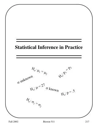
Statistical Inference in Practice. H o : 1 = 2. H o : p 1 = p 2. unknown. H o : = 27. known. H o : p = .5. H o : 1 = 2. Confidence Intervals unknown.

Statistical Inference in Practice
E N D
Presentation Transcript
Statistical Inference in Practice Ho: 1 = 2 Ho: p1 = p2 unknown Ho: = 27 known Ho: p = .5 Ho: 1 = 2 Biostat 511
Confidence Intervals unknown To get a CI for m using the methods outlined previously, we need X and s2. But usually, s is unknown - we only have X and s2. It turns out that even though is normally distributed, is not (quite)! W.S. Gosset worked for Guinness Brewing in Dublin, IR. He was forced to publish under the pseudonym “Student”. In 1908 he derived the distribution of which is now known as Student’s t-distribution. Biostat 511
Normal and t distributions Biostat 511
Confidence Intervals 2 unknown t Distribution When is unknown we replace it with the estimate, s, and use the t-distribution. The statistic has a t-distribution with n-1 degrees of freedom. We can use this distribution to obtain a confidence interval for even when is not known. See MM, table D or display tprob(df,t) A (1-) Confidence Interval for the Population Mean when is unknown Biostat 511
Confidence Intervals - 2 unknown t Distribution - EXAMPLE Given our 30 moms with a mean gestation of 279.5 days and a variance of 28.3 days2, we can now compute a 90% confidence interval for the mean length of pregnancies for second time mothers: Biostat 511
Hypothesis Testing 1-sample Tests: t Test Suppose that we had the cholesterol data but did not know the population variance. Can we still test whether the mean for hypertensives is the same as the general population (211 mg/ml)? Yes! We can use the sample variance to estimate the unknown population variance, then, proceed with the testing using the appropriate t-distribution instead of the standard normal (Z). Biostat 511
Hypothesis Testing 1-sample Tests: t Test Cholesterol Example: Suppose = 220 mg/ml s = 38.6 mg/ml n = 25 H0 : m = 211 mg/ml HA : m¹ 211 mg/ml For an a = 0.05 test we use the critical value determined from the t(24) distribution Since |T| = 1.17 < 2.064 the difference is not statistically significant at the a = 0.05 level and we fail to reject H0. Biostat 511
Hypothesis Testing 1-sample Tests 1. Z-Test: Test of mean with known variance 2. t-Test: Test of mean with unknown variance 3. Test for Binomial Proportion Normal or CLT? Yes No Variance known? Binomial? Yes No Yes No Z test for proportions Nonparametric test Z test t test Biostat 511
Hypothesis Testing 2-sample Motivation 1. Epileptic patients are measured for 4 weeks to record their baseline number of seizures. Patients are then administered treatment with progabide and the number of seizures in the next 4 weeks is recorded. (N = 59 patients). Biostat 511
Hypothesis Testing 2-sample: Paired t Test Assume that we have 2 observations on each person (unit) X1i = the first observation on person i X2i = the second observation on person i Often the hypothesis of interest for paired data looks at the mean difference between these observations. Thus, we base inference on the differences: di = X1i- X2i If we let md = E[di], then the hypothesis of “no treatment effect” can be addressed with the statistics: Biostat 511
Hypothesis Testing 2-sample: Paired t Test Hypotheses: H0: md = 0 HA: md¹ 0 The testing of the hypotheses is then based on the assumed distribution of di under the null hypothesis Or more generally (appealing to the CLT) on the distribution of under the null hypothesis Testing is then based on the statistic which has a t-distribution with n - 1 degrees of freedom. Biostat 511
Hypothesis Testing 2-sample: Paired t Test Returning to the example¼ The hypothesis of no progabide effect becomes H0 : md = 0 The test statistic is The p-value, assuming a 2-sided alternative, is based on the t(58) distribution. P[|T| > 0.29] = 2 ´ P[T < -0.29] = 2 ´ 0.386 (Use tprob or approximate with Z) Biostat 511
A sketch of the p-value calculation is given below: Biostat 511
How about a confidence interval for d? Biostat 511
Hypothesis Testing 2-sample Motivation 2. Suppose that we measure serum iron levels for two groups of children: one group healthy; and one group suffering from cystic fibrosis. We obtain the following data (serum iron measured in mmol/l): Q: Is the mean serum iron level the same for both populations? Q: What is a confidence interval for the mean difference? Biostat 511
Hypothesis Testing 2 Independent Samples We make the following assumptions (justify?) 1. The two samples are independent. 2. The measurements are distributed normally within each population. 3. (or) The sample sizes are “large”. What are the parameters and statistics in this situation? Biostat 511
Hypothesis Testing 2 Independent Samples The hypothesis of interest typically questions the relationship between the two population means. Often, the hypotheses are: H0 : m1 = m2 HA : m1¹m2 Q: What statistic addresses this hypothesis? Q: What is the distribution of this statistic? Biostat 511
This simply comes from two facts that we’ve seen before: 1. sums of independent normals are again normal with mean equal to the sum of the component means and variance equal to the sum of the component variances. 2. The distributions of the sample means. (Aside: why doesn’t this argument work in the paired case?) Biostat 511
Hypothesis Testing 2 Independent Samples For testing the hypotheses H0 : m1 = m2 HA : m1¹m2 We use the standardized test statistic And under the null hypothesis H0 : m1 = m2, we have m1 - m2 = 0so use Biostat 511
Hypothesis Testing 2 Independent Samples To use the test statistic we need to deal with s1 and s2. There are (3) scenarios that we’ll address: 1. s1 and s2 are known. Use these values and T ~ N(0,1) (been there, done that). 2. Assume (unknown). Use and to estimate the common variance s2 and use the appropriate t-distribution after replacing s with the estimate. 3. Assume that the population variances are different and unknown. Use the sample variances to estimate the population variances. We then use an approximate t distribution (ouch!). Biostat 511
Hypothesis Testing 2 Independent Samples - Equal Variances Q: If we are willing to assume that , then how do we use to estimate the common value, s2? A: How about some kind of average? Pooled Estimate of the Variance Biostat 511
Hypothesis Testing 2 Independent Samples - Equal Variances Using this pooled estimate of the variance yields: And under the null hypothesis, H0 : m1 = m2 we use: Biostat 511
Hypothesis Testing 2 Independent Samples - Equal Variances Returning to our example¼ We test the hypothesis of equal means for the two populations, assuming a common variance as follows: H0 : m1 = m2 HA : m1¹m2 Biostat 511
Handle the denominator¼ Now the statistic ¼ For a 2-sided a = 0.05 test we use the critical value: Since |T| = 2.63 > 2.086, we would reject H0 at the a = 0.05 level. Biostat 511
A p-value calculation is shown below: 0.008 0.008 Biostat 511
Hypothesis Testing 2 Independent Samples - Unequal Variances When we aren’t willing to assume that the variances are equal we can still test the population means and use the sample variances. We use the test statistics: Q: What is the distribution of this statistic? A: It’s approximately t-distributed. To use the t-distribution we need the “degrees of freedom”. In this case we use the approximate degrees of freedom (df): Then we round df down to the nearest integer. If the sample sizes are both large, the df will be large and we can simply use Z. Biostat 511
Hypothesis Testing 2 Independent Samples - Unequal Variances Returning to our example¼ We then use the approximate distribution T ~ t(18) Where For a 2-sided a = 0.05 test we compare |T| to the critical value Conclusion? Biostat 511
Hypothesis Testing 2 sample - Equal Variances? • When performing a two-sample t-test (independent or unpaired samples) with unknown population variances we are faced with a choice: • assume pooled variance • assume calculate df In the good ole days, one would look at the data … … and perhaps do a test of the hypothesis Ho: (F-test for variances - see MM sec 7.3). However, this procedure is not “robust” (tends to give incorrect results if the data are not normal) and, in any event, it’s easy to let the computer do the work calculating df. So easiest to just assume all the time. Biostat 511
Confidence Interval - 2 samples We can form a confidence interval for the mean difference d = 1 - 2. In general, use where t* is t distribution with appropriate degrees of freedom. If then use sp and appropriate degrees of freedom. Biostat 511
Summary 1. Testing for 1=2. 2. Testing for 1=2 (not covered in detail). 4. Flowchart for 2 sample test. Normal or CLT? Yes No Inference on means? Binomial? Yes No Yes No Nonparametric test Independent? Inference on var? Independent? Yes No No Yes Yes Variance known? McNemar’s test F test for variances Paired t Expected > 5 No Yes No Variances equal? Yes Z test Fisher’s Eaxct test Yes No 2 sample Z test for proportions or contingency table t test w/ pooled variance t test w/ unequal variance Biostat 511