Semivariogram Basics
The Semivariogram in Remote Sensing: An Introduction P. J. Curran, Remote Sensing of Environment 24: 493-507 (1988). Presented by Dahl Winters Geog 577, April 10, 2007. Semivariogram Basics.

Semivariogram Basics
E N D
Presentation Transcript
The Semivariogram in Remote Sensing: An IntroductionP. J. Curran, Remote Sensing of Environment 24: 493-507 (1988). Presented by Dahl WintersGeog 577, April 10, 2007
Semivariogram Basics The relation between a pair of pixels h intervals apart (lag distance) = the average variance of the differences between all such pairs. The semivarianceS2 for pixels at h distance apart = Within the transect there are m pairs of observations separated by the same lag; their average is given by The above equation, which estimates the average semivariance, measures the dissimilarity between two separated pixels. The larger it is, the less similar the pixels.
More Description The semivariogram is the function that relates semivariance to lag. Lags should be selected that are no longer than 1/5th to 1/3rd the transect length; confidence in the average semivariance estimate increases as the lag becomes shorter.
Interpreting the Semivariogram Urban/agricultural landscapes often have semivariograms with repetitive spatial patterns; the “classic” semivariogram is relatively unusual. The two most common basic forms are the periodic and aspatial semivariograms. Permutations of the classic, periodic, and aspatial forms are the periodic-classic, unbounded, and multifrequency semivariograms. The following examples were done using remotely sensed data from northern England, at 2 m spatial resolution and with 100-pixel transects.
Interpreting the Semivariogram The form of the semivariogram depends on: • the size and spacing of the sample points or the ground resolution elements, • the variable measured in the ground data or the waveband being measured in the remotely sensed data, and • the orientation of the sampling transect. For semivariogram construction, the fine details of spatial dependence are required. Thus, data points recorded closely together at a high spatial resolution are preferred.
Effects of Wavelength and Transect Fortunately, spatial variability within a region is not specific to each variable and waveband, or otherwise separate semivariograms would be needed. Gross spatial features are usually common to all variables and wavebands (they show up in multiple bands). A problem occurs when using remotely sensed data recorded throughout the EM spectrum. A possible workaround is to divide the data into several groups related to physical characteristics of the scene (i.e. water penetration or vegetation reflectance), and construct semivariograms for each group.
Effects of Wavelength and Transect Transect effect: • Transect orientation across rows of different reflectance yields a periodic semivariogram, while transects along these rows do not. Waveband effect: • The periodic semivariogram only appears in wavebands where the rows have contrasting reflectance with the surrounding terrain.
Modeling/Application The most acceptable models for modeling the average semivariance vs. shortest lag distance: spherical, exponential, linear, or combinations of 2 or 3 of these. The linear and spherical models seem to be the most appropriate (Figure 3). Semivariograms can be calculated for any scale of spatial variation (and for any property that is spatially distributed) At all study scales, semivariograms can be used to help with choosing sample units and sample numbers for both remotely sensed and ground data.
Application: Selecting Spatial Resolution of RS Data The spatial resolution of remotely sensed data should not be finer than necessary for the task at hand. To choose a resolution, information is required on the spatial characteristics of the surface being investigated. Example: the size and internal spatial characteristics of fields to be used for calculating per-field radiance values. Field size determines the number of ground resolution elements that will fit inside them. The internal spatial variability determines how small a ground resolution element can be before it detects unnecessary intraparcel variability. The range of a semivariogram defines the distance beyond which ground resolution elements are independent of each other (no autocorrelation). If semivariograms for all wavebands and directions are available, defining a minimum range (i.e. minimum spatial resolution) is straightforward.
Application: Designing a Ground Sampling Scheme Ground data is necessary to calibrate or validate remote sensing data, but it usually has a high degree of sampling error. The ideal number of samples per parcel depends highly on the parcel’s spatial variability. A pilot study can determine this: n = (standard deviation of the measured random sample of points * Student t test value / mean error) ^2 The pilot study procedure assumes the variable of interest is spatially independent (variance is all nugget). If there is spatial dependence, the number of sample points can be much less.
Application: Designing a Ground Sampling Scheme To take advantage of a lower number of samples, we need a sampling grid to ensure that pairs of neighboring sample points are as distant as practical for a fixed sample size and area. This minimizes the information duplication that occurs in random sampling where some sampling points are too close. The procedure to follow: • choose a grid spacing; • use the spacing as the lag; • read off the relevant semivariance from the ground data semivariogram; • use these values to calculate the variance per unit area (the kriging variance). • The kriging variance can be derived in relation to the mean value of the area using:
Conclusions A semivariogram is essentially a plot of spatial dissimilarity over distance. The classic semivariogram is not as common as periodic and periodic-classic semivariograms in urban/agricultural areas, due to the presence of repetitive patterns. The range of a semivariogram is the lag distance beyond which samples are independent of each other (no spatial autocorrelation). Use a semivariogram to determine what the minimum spatial resolution of remote sensing or ground data should be for a particular study.