Basics
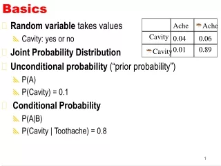
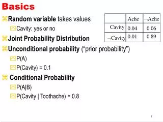
Ache. Ache. Cavity. 0.04 0.06. 0.01 0.89. Cavity. Basics. Random variable takes values Cavity: yes or no Joint Probability Distribution Unconditional probability (“prior probability”) P(A) P(Cavity) = 0.1 Conditional Probability P(A|B) P(Cavity | Toothache) = 0.8.

Basics
E N D
Presentation Transcript
Ache Ache Cavity 0.04 0.06 0.01 0.89 Cavity Basics • Random variable takes values • Cavity: yes or no • Joint Probability Distribution • Unconditional probability (“prior probability”) • P(A) • P(Cavity) = 0.1 • Conditional Probability • P(A|B) • P(Cavity | Toothache) = 0.8
C A P Prob F F F 0.534 F F T 0.356 F T F 0.006 F T T 0.004 T F F 0.048 T F T 0.012 T T F 0.032 T T T 0.008 Conditional Independence • “A and P are independent” • P(A) = P(A | P) and P(P) = P(P | A) • Can determine directly from JPD • Powerful, but rare(I.e. not true here) • “A and P are independent given C” • P(A|P,C) = P(A|C) and P(P|C) = P(P|A,C) • Still powerful, and also common • E.g. suppose • Cavities causes aches • Cavities causes probe to catch Ache Cavity Probe
C A P Prob F F F 0.534 F F T 0.356 F T F 0.006 F T T 0.004 T F F 0.012 T F T 0.048 T T F 0.008 T T T 0.032 Conditional Independence • “A and P are independent given C” • P(A | P,C) = P(A | C) and also P(P | A,C) = P(P | C)
Suppose C=True P(A|P,C) = 0.032/(0.032+0.048) = 0.032/0.080 = 0.4
P(A|C) = 0.032+0.008/ (0.048+0.012+0.032+0.008) = 0.04 / 0.1 = 0.4
Why Conditional Independence? • Suppose we want to compute • p(X1, X2,…,Xn) • And we know that: • P(Xi | Xi+1,…,Xn) = P(Xi | Xi+1) • Then, • p(X1, X2,…,Xn)= p(X1|X2) x … x P(Xn-1|Xn) P(Xn) • And you can specify the JPD using linearly sized table, instead of exponential. • Important intuition for the savings obtained by Bayes Nets.
Summary so Far • Bayesian updating • Probabilities as degree of belief (subjective) • Belief updating by conditioning • Prob(H) Prob(H|E1) Prob(H|E1, E2) ... • Basic form of Bayes’ rule • Prob(H | E) = Prob(E | H) P(H) / Prob(E) • Conditional independence • Knowing the value of Cavity renders Probe Catching probabilistically independent of Ache • General form of this relationship: knowing the values of all the variables in some separator set S renders the variables in set A independent of the variables in B. Prob(A|B,S) = Prob(A|S) • Graphical Representation...
Computational Models for Probabilistic Reasoning • What we want • a “probabilistic knowledge base” where domain knowledge is represented by propositions, unconditional, and conditional probabilities • an inference engine that will computeProb(formula | “all evidence collected so far”) • Problems • elicitation: what parameters do we need to ensure a complete and consistent knowledge base? • computation: how do we compute the probabilities efficiently? • Belief nets (“Bayes nets”) = Answer (to both problems) • a representation that makes structure (dependencies and independence assumptions) explicit
Causality • Probability theory represents correlation • Absolutely no notion of causality • Smoking and cancer are correlated • Bayes nets use directed arcs to represent causality • Write only (significant) direct causal effects • Can lead to much smaller encoding than full JPD • Many Bayes nets correspond to the same JPD • Some may be simpler than others
C P(A) T 0.4 F 0.02 P(C) .01 C P(P) T 0.8 F 0.4 Compact Encoding • Can exploit causality to encode joint probability distribution with many fewer numbers C A P Prob F F F 0.534 F F T 0.356 F T F 0.006 F T T 0.004 T F F 0.012 T F T 0.048 T T F 0.008 T T T 0.032 Ache Cavity Probe Catches
P(A) .05 A Different Network Ache A T T F F P T F T F P(C) .888889 .571429 .118812 .021622 Cavity Probe Catches A P(P) T 0.72 F 0.425263
Creating a Network 1: Bayes net = representation of a JPD 2: Bayes net = set of cond. independence statements • If create correct structure • Ie one representing causality • Then get a good network • I.e. one that’s small = easy to compute with • One that is easy to fill in numbers
Example My house alarm system just sounded (A). Both an earthquake (E) and a burglary (B) could set it off. John will probably hear the alarm; if so he’ll call (J). But sometimes John calls even when the alarm is silent Mary might hear the alarm and call too (M), but not as reliably We could be assured a complete and consistent model by fully specifying the joint distribution: Prob(A, E, B, J, M) Prob(A, E, B, J, ~M) etc.
Structural Models Instead of starting with numbers, we will start with structural relationships among the variables direct causal relationship from Earthquake to Alarm direct causal relationship from Burglar to Alarm direct causal relationship from Alarm to JohnCall Earthquake and Burglar tend to occur independently etc.
Possible Bayes Network Earthquake Burglary Alarm MaryCalls JohnCalls
Graphical Models and Problem Parameters • What probabilities need I specify to ensure a complete, consistent model given? • the variables one has identified • the dependence and independence relationships one has specified by building a graph structure • Answer • provide an unconditional (prior) probability for every node in the graph with no parents • for all remaining, provide a conditional probability table • Prob(Child | Parent1, Parent2, Parent3) for all possible combination of Parent1, Parent2, Parent3 values
P(E) .002 P(B) .001 B T T F F E T F T F P(A) .95 .94 .29 .01 A T F P(J) .90 .05 A T F P(M) .70 .01 Complete Bayes Network Earthquake Burglary Alarm MaryCalls JohnCalls
NOISY-OR: A Common Simple Model Form • Earthquake and Burglary are “independently cumulative” causes of Alarm • E causes A with probability p1 • B causes A with probability p2 • the “independently cumulative” assumption saysProb(A | E, B) = p1 + p2 - p1p2 • with possibly a “spontaneous causality” parameter Prob(A | ~E, ~B) = p3 • A noisy-OR model with M causes has M+1 parameters while the full model has 2M
More Complex Example My house alarm system just sounded (A). Both an earthquake (E) and a burglary (B) could set it off. Earthquakes tend to be reported on the radio (R). My neighbor will usually call me (N) if he (thinks he) sees a burglar. The police (P) sometimes respond when the alarm sounds. What structure is best?
Structural relationships imply statements about probabilistic independence P is independent from E and Bprovided we know the value of A. A is independent of Nprovided we know the value of B. Earthquake Burglary Radio Alarm Neighbor Police A First-Cut Graphical Model
Structural Relationships and Independence • The basic independence assumption (simplified version): • two nodes X and Y are probabilistically independent conditioned on E if every undirected path from X to Y is d-separated by E • every undirected path from X to Y is blocked by E • if there is a node Z for which one of three conditions hold • Z is in E and Z has one incoming arrow on the path and one outgoing arrow • Z is in E and both arrows lead out of Z • neither Z nor any descendent of Z is in E, and both arrows lead into Z
E Z X Z Y Z Z Cond. Independence in Bayes Nets • If a set E d-separates X and Y • Then X and Y are cond. independent given E • Set E d-separates X and Y if every undirected path between X and Y has a node Z such that, either Why important??? P(A | B,C) = P(A) P(B|A) P(C|A)
Inference • Given exact values for evidence variables • Compute posterior probability of query variable • Diagnostic • effects to causes • Causal • causes to effects • Intercausal • between causes of common effect • explaining away • Mixed P(E) .002 P(B) .001 Earthq Burglary B T T F F E T F T F P(A) .95 .94 .29 .01 Alarm A T F A T F P(J) .90 .05 P(M) .70 .01 MaryCall JonCalls
Algorithm • In general: NP Complete • Easy for polytrees • I.e. only one undirected path between nodes • Express P(X|E) by • 1. Recursively passing support from ancestor down • “Causal support” • 2. Recursively calc contribution from descendants up • “Evidential support” • Speed: linear in the number of nodes (in polytree)
P(B) .001 Burglary P(A) .95 .01 B T F Alarm Simplest Causal Case • Suppose know Burglary • Want to know probability of alarm • P(A|B) = 0.95
Suppose know Alarm ringing & want to know: Burglary? I.e. want P(B|A) P(B) .001 Burglary P(A) .95 .01 B T F Alarm Simplest Diagnostic Case P(B|A) =P(A|B) P(B) / P(A) But we don’t know P(A) 1 =P(B|A)+P(~B|A) 1 =P(A|B)P(B)/P(A) + P(A|~B)P(~B)/P(A) 1 =[P(A|B)P(B) + P(A|~B)P(~B)] / P(A) P(A) = P(A|B)P(B) + P(A|~B)P(~B) P(B | A) = P(A|B) P(B) / [P(A|B)P(B) + P(A|~B)P(~B)] = .95*.001 / [.95*.001 + .01*.999] =0.087
+ Ex • Express P(X | E) in terms of contributions of Ex+ and Ex- - Ex General Case Um U1 ... X • Compute contrib of Ex+ by computing effect of parents of X (recursion!) • Compute contrib of Ex- by ... Z1j Znj Yn ... Y1