Download
1 / 24
240 likes | 462 Vues
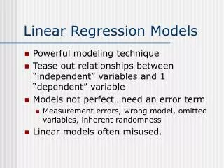
Linear Regression Models. Powerful modeling technique Tease out relationships between “independent” variables and 1 “dependent” variable Models not perfect…need an error term Measurement errors, wrong model, omitted variables, inherent randomness Linear models often misused.

E N D
Linear Regression Models • Powerful modeling technique • Tease out relationships between “independent” variables and 1 “dependent” variable • Models not perfect…need an error term • Measurement errors, wrong model, omitted variables, inherent randomness • Linear models often misused.
Example: Lake Water Quality • Chlorophyll-a (C) widely used indicator – measure of eutrophication • Nitrogen (N) associated with eutrophication • Q: Golf Course Development. Nitrogen expected to . By how much will C increase/decrease? • How should we proceed?
A “Better” Model • Explain (single) regression line (model?). • Neg. relationship suggests a problem. • Omitted variable: Phosphorus (P) • Want to tease out effect of N, P separately. • Write a Multiple Linear Regression Model: • Model designed to “tease out” effect of N and effect of P, separately, on C. • (**) Define and interpret variables, parameters.
Estimation • Use data to estimate parameter values that give “best fit”: b0=-9.4, b1=0.3, b2=1.2 • Answer: A one unit increase in N, results in about a 1.2 unit increase in C. • Importance: Omitting phosphorus from model introduced significant bias!!!
Question: US Gas Consumption • Gasoline consumption produces many negative byproducts. • Policy may be directed at increasing the price of gas to reduce consumption. • But what is effect of price change? • Question: What is the price elasticity of demand for gasoline in the U.S.?
Gas Data Cont’d • Gas consumption increases through time. But no info here about price. • Next plot shows (+) relationship between gas price and gas consumption. • Note opposite of demand curve. • Something is wrong here… • Just as in Eutrophication problem, may have omitted important variables. • May have other problems, too.
The OLS “Estimator” • Estimator: A rule or strategy for using data to estimate an unknown parameter. Defined before the data are drawn. • Ordinary Least Squares (OLS) estimator finds value of parameter that minimizes sum of squared deviations (see C vs. N plot) • Several assumptions for OLS estimator to apply to a model
Linear Model • The model must be linear • Linear in parameters, not in variables. • Difference between parameter, variable. • Examples:
Transforming Models • Previous “Ricker” model is non-linear (in the parameter). • Sometimes, can transform model so linear. • When plot, graph is nonlinear. • Take log of both sides, giving:
CLRM: Assumption 1 • Dependent variable (Y) is function of specific set of independent variables (X’s). • Linear in parameters • Additive error • Coefficients are constant but unknown • Violations called “specification errors”, e.g. • Wrong regressors (a.k.a. indep. vars; X’s) • Nonlinearity • Changing parameters (e.g. through time)
CLRM: Assumption 2 • Disturbances (ei’s) are independently and identically distributed ~ (0,s2) • Typically we assume ei~ N(0,s2) • Mean = 0 • Constant variance, s2 (but unknown) • Errors uncorrelated with one another • Example of violations: • Measurement Bias (seep gas flux) • Heteroskedasticity (variance differs). • Autocorrelated Errors (disturbances correlated)
CLRM: Assumption 3 • It is possible to repeat the sample with same independent variables. • If had same levels of explanatory vars, would it be possible to generate same value of Y? • Common Violations: • Errors in variables – measurement error in X. • Autoregression – when lagged dependent variable should be independent variable • Simultaneous Equations – several relationships act jointly.
Properties of Estimators • Estimators have many properties. • “6” is an estimator, but not a very good one. • Two main properties we care about: • Unbiased: The expected distance of estimator from thing it is estimating is 0. • Efficient: Small variance (spread) • “6” is biased, but has a very small variance (zero). • OLS estimator is unbiased and has minimum variance of all unbiased estimators.
Correlation vs. Causation • Now we know just enough to be dangerous! • Can estimate how any set of variables affects some other variable….Very Powerful. • Problem is: Correlation doesn’t imply Causation! …. Why Data Mining is bad. • Chicken production, Global CO2. • May be “spurious” (no underlying relationship) • Difficult to tease out statistically. • “Granger Causality”
Guide to Model Specification • Start with theory to generate model • Check assumptions of CLRM • Collect and plot data • Estimate model, test restrictions • Possibly perform Box-Cox transform • Check R2, and “Adjusted R2” • Plot residuals – look for patterns • Seek explanations for patterns
What’s a Residual? • General form of linear model: • Graphically on board.
Residuals vs. Fit Normal Quantile Plot Residual Plots
Back to Gasoline Consumption • Recall, interested in how gas consumption is affected by price increase (say $0.10/gal.) • Variables: • Gas consumption per capita (G) • Gas price (Pg) • Income (Y) • New car price (Pnc) • Used car price (Puc)
2 Alternative Specifications • Linear specification: • Log-log specification (often used with economic data) • One way to test specification is Box-Cox Transform (see 3 lectures back)
Results of Linear Model • Parameter estimate, (p-value of t-test). • Low p-value: “statistically significant” • R2 measures goodness of fit of model. • Low p-value of F statistic means model has explanatory power.
Answer to Question • A 1 unit increase in price leads to a .04 unit decrease in gas consumption. • Units are: G(1000 gallons), Pg($). • So, a $0.10 increase in gas price leads to, on average, a 4 gallon decrease in gas consumption…not much!