Linear Regression Models
Linear Regression Models. Based on Chapter 3 of Hastie, Tibshirani and Friedman Slides by David Madigan. Linear Regression Models. Here the X ’s might be:. Raw predictor variables (continuous or coded-categorical) Transformed predictors ( X 4 =log X 3 )


Linear Regression Models
E N D
Presentation Transcript
Linear Regression Models Based on Chapter 3 of Hastie, Tibshirani and Friedman Slides by David Madigan
Linear Regression Models Here the X’s might be: • Raw predictor variables (continuous or coded-categorical) • Transformed predictors (X4=log X3) • Basis expansions (X4=X32,X5=X33, etc.) • Interactions (X4=X2X3 ) Popular choice for estimation is least squares:
Least Squares hat matrix Often assume that the Y’s are independent and normally distributed, leading to various classical statistical tests and confidence intervals
Gauss-Markov Theorem Consider any linear combination of the ’s: The least squares estimate of is: If the linear model is correct, this estimate is unbiased (X fixed): Gauss-Markov states that for any other linear unbiased estimator : Of course, there might be a biased estimator with lower MSE…
bias-variance For any estimator : bias Note MSE closely related to prediction error:
Too Many Predictors? When there are lots of X’s, get models with high variance and prediction suffers. Three “solutions:” • Subset selection • Shrinkage/Ridge Regression • Derived Inputs Score: AIC, BIC, etc. All-subsets + leaps-and-bounds, Stepwise methods,
Subset Selection • Standard “all-subsets” finds the subset of size k, k=1,…,p, that minimizes RSS: • Choice of subset size requires tradeoff – AIC, BIC, marginal likelihood, cross-validation, etc. • “Leaps and bounds” is an efficient algorithm to do all-subsets
Cross-Validation • e.g. 10-fold cross-validation: • Randomly divide the data into ten parts • Train model using 9 tenths and compute prediction error on the remaining 1 tenth • Do these for each 1 tenth of the data • Average the 10 prediction error estimates “One standard error rule” pick the simplest model within one standard error of the minimum
Shrinkage Methods • Subset selection is a discrete process – individual variables are either in or out • This method can have high variance – a different dataset from the same source can result in a totally different model • Shrinkage methods allow a variable to be partly included in the model. That is, the variable is included but with a shrunken co-efficient.
Ridge Regression subject to: Equivalently: This leads to: Choose by cross-validation. Predictors should be centered. works even when XTX is singular
The Lasso subject to: Quadratic programming algorithm needed to solve for the parameter estimates. Choose s via cross-validation. q=0: var. sel. q=1: lasso q=2: ridge Learn q?
Principal Component Regression Consider a an eigen-decomposition of XTX (and hence the covariance matrix of X): The eigenvectors vj are called the principal components of X D is diagonal with entries d1 ≥ d2 ≥… ≥dp has largest sample variance amongst all normalized linear combinations of the columns of X has largest sample variance amongst all normalized linear combinations of the columns of X subject to being orthogonal to all the earlier ones
Principal Component Regression PC Regression regresses on the first M principal components where M<p Similar to ridge regression in some respects – see HTF, p.66