Some Multivariate techniques Principal components analysis (PCA) Factor analysis (FA) Structural equation models (SEM) A
Some Multivariate techniques Principal components analysis (PCA) Factor analysis (FA) Structural equation models (SEM) Applications : Personality. Boulder March 2006. Dorret I. Boomsma Danielle Dick Marleen de Moor Mike Neale Conor Dolan. Presentation in dorret2006.

Some Multivariate techniques Principal components analysis (PCA) Factor analysis (FA) Structural equation models (SEM) A
E N D
Presentation Transcript
Some Multivariate techniquesPrincipal components analysis (PCA)Factor analysis (FA)Structural equation models (SEM)Applications: Personality Boulder March 2006 Dorret I. Boomsma Danielle Dick Marleen de Moor Mike Neale Conor Dolan Presentation in dorret\2006
Multivariate statistical methods; for example -Multiple regression -Fixed effects (M)ANOVA -Random effects (M)ANOVA Factor analysis / PCA Time series (ARMA) Path / LISREL models
Multiple regression x e y x e y x predictors (independent), e residuals, y dependent; both x and y are observed x e y x
Factor analysis:measured and unmeasured (latent) variables. Measured variables can be “indicators” of unobserved traits.
Path model / SEM model Latent traits can influence other latent traits
Measurement and causal models in non-experimental research • Principal component analysis (PCA) • Exploratory factor analysis (EFA) • Confirmatory factor analysis (CFA) • Structural equation models (SEM) • Path analysis These techniques are used to analyze multivariate data that have been collected in non-experimental designs and often involve latent constructs that are not directly observed. These latent constructs underlie the observed variables and account for inter-correlations between variables.
Models in non-experimental research All models specify a covariance matrix S and means vector m: S = LYLt + Q total covariance matrix [S] = factor variance [LYLt ] + residual variance [Q] means vector m can be modeled as a function of other (measured) traits e.g. sex, age, cohort, SES
Outline • Cholesky decomposition • PCA (eigenvalues) • Factor models (1,..4 factors) • Application to personality data • Scripts for Mx, [Mplus, Lisrel]
Application: personality • Personality (Gray 1999): a person’s general style of interacting with the world, especially with other people – whether one is withdrawn or outgoing, excitable or placid, conscientious or careless, kind or stern. • Is there one underlying factor? • Two, three, more?
Personality: Big 3, Big 5, Big 9? Big 3Big5Big 9MPQ scales Extraversion Extraversion Affiliation Social Closeness Potency Social Potency Achievement Achievement Psychoticism Conscientious Dependability Control Agreeableness Agreeableness Aggression Neuroticism Neuroticism Adjustment Stress Reaction Openness Intellectance Absorption Individualism Locus of Control
Data: Neuroticism, Somatic anxiety, Trait Anxiety, Beck Depression, Anxious/Depressed, Disinhibition, Boredom susceptibility, Thrill seeking, Experience seeking, Extraversion, Type-A behavior, Trait Anger, Test attitude (13 variables) Software scripts • Mx MxPersonality (also includes data) • (Mplus) Mplus • (Lisrel) Lisrel • Copy from dorret\2006
Cholesky decomposition for 13 personality traits Cholesky decomposition: S = Q Q’ where Q = lower diagonal (triangular) For example, if S is 3 x 3, then Q looks like: f1l 0 0 f21 f22 0 f31 f32 f33 I.e. # factors = # variables, this approach gives a transformation of S; completely determinate.
Subjects: Birth cohorts (1909 – 1989) Four data sets were created: 1 Old male (N = 1305) 2 Young male (N = 1071) 3 Old female (N = 1426) 4 Young female (N = 1070) What is the structure of personality? Is it the same in all datasets? Total sample: 46% male, 54% female
Application: Analysis of Personality in twins, spouses, sibs,parents from Adult Netherlands Twin Register: longitudinal participation Data from multiple occasions were averaged for each subject; Around 1000 Ss were quasi-randomly selected for each sex-age group Because it is March 8, we use data set 3 (personShort sexcoh3.dat)
dorret\2006\Mxpersonality (docu.doc) • Datafiles for Mx (and other programs; free format) • personShort_sexcoh1.dat old males N=1035 (average yr birth 1943) • personShort_sexcoh2.dat young males N=1071 (1971) • personShort_sexcoh3.dat old females N=1426 (1945) • personShort_sexcoh4.dat young females N=1070 (1973) • Variables (53 traits): (averaged over time survey 1 – 6) trappreg trappext sex1to6 gbdjr twzyg halfsib id_2twns drieli: demographics neu ext nso tat tas es bs dis sbl jas angs boos bdi : personality ysw ytrg ysom ydep ysoc ydnk yatt ydel yagg yoth yint yext ytot yocd: YASR cfq mem dist blu nam fob blfob scfob agfob hap sat self imp cont chck urg obs com: other • Mx Jobs • Cholesky 13vars.mx : cholesky decomposition (saturated model) • Eigen 13vars.mx: eigenvalue decomposition of computed correlation matrix (also saturated model) • Fa 1 factors.mx: 1 factor model • Fa 2 factors.mx : 2 factor model • Fa 3 factors.mx: 3 factor model (constraint on loading) • Fa 4 factors.mx: 1 general factor, plus 3 trait factors • Fa 3 factors constraint dorret.mx • Fa 3 factors constraint dorret.mx: alternative constraint to identify the model
title cholesky for sex/age groups data ng=1 Ni=53 !8 demographics, 13 scales, 14 yasr, 18 extra missing=-1.00 !personality missing = -1.00 rectangular file =personShort_sexcoh3.dat labels trappreg trappext sex1to6 gbdjr twzyg halfsib id_2twns drieli neu ext nso etc. Select NEU NSO ANX BDI YDEP TAS ES BS DIS EXT JAS ANGER TAT / begin matrices; A lower 13 13 free !common factors M full 1 13 free !means end matrices; covariance A*A'/ means M / start 1.5 all etc. option nd=2 end
NEU NSO ANX BDI YDEP TAS ES BS DIS EXT JAS ANGER TAT / MATRIX A: This is a LOWER TRIANGULAR matrix of order 13 by 13 • 23.74 • 3.55 4.42 • 6.89 0.96 5.34 • 1.70 0.72 0.80 2.36 • 2.79 0.32 0.68 -0.08 2.87 • -0.30 0.03 -0.01 0.16 0.18 7.11 • 0.28 0.13 0.17 -0.04 0.24 3.32 6.03 • 1.29 -0.08 0.30 -0.15 -0.09 0.96 1.52 6.01 • 0.83 -0.07 0.35 -0.30 0.15 1.97 0.91 1.16 5.23 • -4.06 -0.11 -1.41 -0.20 -0.90 2.04 1.07 3.14 0.94 14.06 • 1.85 -0.02 0.70 -0.28 0.01 0.47 0.00 0.43 -0.08 1.11 3.98 • 1.86 -0.09 0.80 -0.49 -0.18 0.13 0.04 0.21 0.18 0.51 0.97 3.36 • -1.82 0.16 -0.34 0.02 -1.26 -0.16 -0.46 -0.80 -0.53 -1.21 -1.20 -1.64 7.71
To interpret the solution, standardize the factor loadings both with respect to the latent and the observed variables.In most models, the latent variables have unit variance;standardize the loadings by the variance of the observed variables (e.g. λ21 is divided by the SD of P2) F5 F1 F2 F3 F4 P3 P5 P1 P4 P2
Group 2 in Cholesky script Calculate Standardized Solution Calculation Matrices = Group 1 I Iden 13 13 End Matrices; Begin Algebra; S=(\sqrt(I.R))~; ! diagonal matrix of standard deviations P=S*A; ! standardized estimates for factors loadings End Algebra; End (R=(A*A'). i.e. R has variances on the diagonal)
Standardized solution: standardized loadingsNEU NSO ANX BDI YDEP TAS ES BS DIS EXT JAS ANGER TAT / • 1.00 • 0.63 0.78 • 0.79 0.11 0.61 • 0.55 0.23 0.26 0.76 • 0.69 0.08 0.17 -0.02 0.70 • -0.04 0.00 0.00 0.02 0.03 0.99 • 0.04 0.02 0.02 -0.01 0.04 0.48 0.87 • 0.20 -0.01 0.05 -0.02 -0.01 0.15 0.24 0.94 • 0.14 -0.01 0.06 -0.05 0.02 0.34 0.15 0.20 0.89 • -0.27 -0.01 -0.09 -0.01 -0.06 0.13 0.07 0.21 0.06 0.92 • 0.40 0.00 0.15 -0.06 0.00 0.10 0.00 0.09 -0.02 0.240.86 • 0.45 -0.02 0.19 -0.12 -0.04 0.03 0.01 0.05 0.04 0.12 0.24 0.82 • -0.22 0.02 -0.04 0.00 -0.15 -0.02 -0.05 -0.09 -0.06 -0.14 -0.14 -0.19 0.91
NEU NSO ANX BDI YDEP TAS ES BS DIS EXT JAS ANGER TAT / • Your model has104 estimated parameters : • 13 means • 13*14/2 = 91 factor loadings • -2 times log-likelihood of data >>>108482.118
Eigenvalues, eigenvectors & principal component analyses (PCA) 1) data reduction technique2) form of factor analysis3) very useful transformation
Principal components analysis (PCA) PCA is used to reduce large set of variables into a smaller number of uncorrelated components. Orthogonal transformation of a set of variables (x) into a set of uncorrelated variables (y) called principal components that are linear functions of the x-variates. The first principal component accounts for as much of the variability in the data as possible, and each succeeding component accounts for as much of the remaining variability as possible.
Principal component analysis of 13 personality / psychopathology inventories: 3 eigenvalues > 1(Dutch adolescent and young adult twins, data 1991-1993; SPSS)
Principal components analysis (PCA) PCA gives a transformation of the correlation matrix R and is a completely determinate model. R (q x q) = P D P’, where P = q x q orthogonal matrix of eigenvectors D = diagonal matrix (containing eigenvalues) y = P’ x and the variance of yj is pj The first principal component y1 = p11x1 + p12x2 + ... + p1qxq The second principal component y2 = p21x1 + p22x2 + ... + p2qxq etc. [p11, p12, … , p1q] is the first eigenvector d11 is the first eigenvalue (variance associated with y1)
Principal components analysis (PCA) The principal components are linear combinations of the x-variables which maximize the variance of the linear combination and which have zero covariance with the other principal components. There are exactly q such linear combinations (if R is positive definite). Typically, the first few of them explain most of the variance in the original data. So instead of working with X1, X2, ..., Xq, you would perform PCA and then use only Y1 and Y2, in a subsequent analysis.
PCA, Identifying constraints: transformation unique Characteristics: 1) var(dij) is maximal 2) dij is uncorrelated with dkj are ensured by imposing the constraint: PP' = P'P = I (where ' stands for transpose)
Principal components analysis (PCA) The objective of PCA usually is not to account for covariances among variables, but to summarize the information in the data into a smaller number of (orthogonal) variables. No distinction is made between common and unique variances. One advantage is that factor scores can be computed directly and need not to be estimated. ‑ H. Hotelling (1933): Analysis of a complex of statistical variables into principal component. Journal Educational Psychology, 417-441, 498-520
PCA Primarily data reduction technique, but often used as form of exploratory factor analysis: Scale dependent (use only correlation matrices)! Not a “testable” model, no statistical inference Number of components based on rules of thumb (e.g. # of eigenvalues > 1)
title eigen values data ng=1 Ni=53 missing=-1.00 rectangular file =personShort_sexcoh3.dat labels trappreg trappext sex1to6 gbdjr twzyg halfsib id_2twns drieli neu ext nso tat tas etc. Select NEU NSO ANX BDI YDEP TAS ES BS DIS EXT JAS ANGER TAT / begin matrices; R stand 13 13 free !correlation matrix S diag 13 13 free !standard deviations M full 1 13 free !means end matrices; begin algebra; E = \eval(R); !eigenvalues of R V = \evec(R); !eigenvectors of R end algebra; covariance S*R*S'/ means M / start 0.5 all etc. end
Correlations NEU NSO ANX BDI YDEP TAS ES BS DIS EXT JAS ANGER TAT / MATRIX R: This is a STANDARDISED matrix of order 13 by 13 • 1.000 • 0.625 1.000 • 0.785 0.576 1.000 • 0.548 0.523 0.612 1.000 • 0.685 0.490 0.648 0.421 1.000 • -0.041 -0.023 -0.033 -0.005 -0.011 1.000 • 0.041 0.040 0.049 0.028 0.059 0.480 1.000 • 0.202 0.116 0.186 0.102 0.136 0.140 0.288 1.000 • 0.142 0.080 0.146 0.052 0.125 0.329 0.305 0.306 1.00 • -0.266 -0.172 -0.266 -0.181 -0.239 0.143 0.110 0.172 0.108 • 0.400 0.247 0.406 0.211 0.301 0.083 0.070 0.191 • 0.451 0.265 0.470 0.201 0.312 0.009 0.045 0.159 ETC • -0.216 -0.120 -0.192 -0.123 -0.258 -0.013 -0.071 -0.148
Eigenvalues • MATRIX E: This is a computed FULL matrix of order 13 by 1, [=\EVAL(R)] • 1 0.200 • 2 0.263 • 3 0.451 • 4 0.457 • 5 0.518 • 6 0.549 • 7 0.677 • 8 0.747 • 9 0.824 • 10 0.856 • 11 1.300 • 12 2.052 • 13 4.106 What is the fit of this model? It is the same as for Cholesky Both are saturated models
Principal components analysis (PCA): S = P D P' = P* P*' where S = observed covariance matrix P'P = I (eigenvectors) D = diagonal matrix (containing eigenvalues) P* = P (D1/2) Cholesky decomposition: S = Q Q’ where Q = lower diagonal (triangular) For example, if S is 3 x 3, then Q looks like: f1l 0 0 f21 f22 0 f31 f32 f33 If # factors = # variables, Q may be rotated to P*. Both approaches give a transformation of S. Both are completely determinate.
PCA is based on the eigenvalue decomposition. S=P*D*P’ If the first component approximates S: SP1*D1*P1’ SP1*P1’, P1 = P1*D11/2 It resembles the common factor model SS=L*L’ +Q, LP1
pc1 h pc2 pc3 pc4 y1 y2 y3 y4 y1 y2 y3 y4 If pc1 is large, in the sense that it accounts for much variance h pc1 => y1 y2 y3 y4 y1 y2 y3 y4 Then it resembles the common factor model (without unique variances)
Factor analysis Aims at accounting for covariances among observed variables / traits in terms of a smaller number of latent variates or common factors. Factor Model: x = f + e, where x = observed variables f = (unobserved) factor score(s) e = unique factor / error = matrix of factor loadings
Factor analysis: Regression of observed variables (x or y) on latent variables (f or η) One factor model with specifics
Factor analysis • Factor Model: x = f + e, • With covariance matrix: = ' + • where = covariance matrix • = matrix of factor loadings • = correlation matrix of factor scores • = (diagonal) matrix of unique variances • To estimate factor loadings we do not need to know the individual factor scores, as the expectation for only consists of , , and . • C. Spearman (1904): General intelligence, objectively determined and measured. American Journal of Psychology, 201-293 • L.L. Thurstone (1947): Multiple Factor Analysis, University of Chicago Press
One factor model for personality? • Take the cholesky script and modify it into a 1 factor model (include unique variances for each of the 13 variables) • Alternatively, use the FA 1 factors.mx script • NB think about starting values (look at the output of eigen 13 vars.mx for trait variances)
Confirmatory factor analysis An initial model (i.e. a matrix of factor loadings) for a confirmatory factor analysis may be specified when for example: • its elements have been obtained from a previous analysis in another sample. • its elements are described by a clinical model or a theoretical process (such as a simplex model for repeated measures).
Mx script for 1 factor model title factor data ng=1 Ni=53 missing=-1.00 rectangular file =personShort_sexcoh3.dat labels trappreg trappext sex1to6 gbdjr twzyg halfsib id_2twns drieli neu ext ETC Select NEU NSO ANX BDI YDEP TAS ES BS DIS EXT JAS ANGER TAT / begin matrices; A full 13 1 free !common factors B iden 1 1 !variance common factors M full 13 1 free !means E diag 13 13 free !unique factors (SD) end matrices; specify A 1 2 3 4 5 6 7 8 9 10 11 12 13 covariance A*B*A' + E*E'/ means M / Starting values end
Mx output for 1 factor model Unique loadings are found on the Diagonal of E. Means are found in M matrix loadings 1 • neu 21.3153 • nso 3.7950 • anx 7.7286 • bdi 1.9810 • ydep 3.0278 • tas -0.1530 • es 0.4620 • bs 1.4337 • dis 0.9883 • ext -3.9329 • jas 2.1012 • anger 2.1103 • tat -2.1191 Your model has 39 estimated parameters -2 times log-likelihood of data 109907.192 13 means 13 loadings on the common factor 13 unique factor loadings
Factor analysis • Factor Model: x = f + e, • Covariance matrix: = ' + • Because the latent factors do not have a “natural” scale, the user needs to scale them. For example: • If = I: = ' + • factors are standardized to have unit variance • factors are independent • Another way to scale the latent factors would be to constrain one of the factor loadings.
In confirmatory factor analysis: • a model is constructed in advance • that specifies the number of (latent) factors • that specifies the pattern of loadings on the factors • that specifies the pattern of unique variances specific to each observation • measurement errors may be correlated • factor loadings can be constrained to be zero (or any other value) • covariances among latent factors can be estimated or constrained • multiple group analysis is possible • We can TEST if these constraints are consistent with the data.
Distinctions between exploratory (SPSS/SAS) and confirmatory factor analysis (LISREL/Mx) • In exploratory factor analysis: • no model that specifies the number of latent factors • no hypotheses about factor loadings (usually all variables load on all factors, factor loadings cannot be constrained) • no hypotheses about interfactor correlations (either no correlations or all factors are correlated) • unique factors must be uncorrelated • all observed variables must have specific variances • no multiple group analysis possible • under-identification of parameters
f1 f2 f3 X1 X2 X3 X4 X5 X6 X7 e1 e2 e3 e4 e5 e6 e7 Exploratory Factor Model
f1 f2 f3 X1 X2 X3 X4 X5 X6 X7 e1 e2 e3 e4 e5 e7 Confirmatory Factor Model
Confirmatory factor analysis A maximum likelihood method for estimating the parameters in the model has been developed by Jöreskog and Lawley (1968) and Jöreskog (1969). ML provides a test of the significance of the parameter estimates and of goodness-of-fit of the model. Several computer programs (Mx, LISREL, EQS) are available. • K.G. Jöreskog, D.N. Lawley (1968): New Methods in maximum likelihood factor analysis. British Journal of Mathematical and Statistical Psychology, 85-96 • K.G. Jöreskog (1969): A general approach to confirmatory maximum likelihood factor analysis Psychometrika, 183-202 • D.N. Lawley, A.E. Maxwell (1971): Factor Analysis as a Statistical Method. Butterworths, London • S.A. Mulaik (1972): The Foundations of Factor analysis, McGraw-Hill Book Company, New York • J Scott Long (1983): Confirmatory Factor Analysis, Sage
Structural equation models Sometimes x = f + e is referred to as the measurement model, and the part of the model that specifies relations among latent factors as the covariance structure model, or the structural equation model.
f1 f2 f3 X4 X7 X5 X2 X1 X3 X6 e5 e7 e4 e3 e2 e1 Structural Model