Download
1 / 56
570 likes | 738 Vues
Phlebotomy Training for M-III Students: Statistical Analysis of Test Results. Richard A. McPherson, M.D., M.S. Phlebotomy Training 2001-2008. Exercise offered to third year medical students as part of orientation every year since 2001.

E N D
Phlebotomy Training for M-III Students: Statistical Analysis of Test Results Richard A. McPherson, M.D., M.S.
Phlebotomy Training 2001-2008 • Exercise offered to third year medical students as part of orientation every year since 2001. • This is the third year that phlebotomy training was mandatory. • Other exercises offered in IV/Foley catheter placement.
Numbers of Students Submitting Blood Specimens Each year • 2001 103 • 2002 83 • 2003 102 • 2004 87 • 2005 98 • 2006 150 • 2007 147 • 2008 134 • Total 904
Phlebotomy Training 2008 • Wednesday, July 23, 2008 in three separate sessions held in the Medical Sciences Building at 1, 2 and 3 PM. • A total of 153 students attended the exercise in which each student collected two tubes of blood on a partner. • Specimens were successfully collected from 134 students and submitted to the laboratory for simple chemical and hematological measurements. • The students’ own results were provided to them with a unique identifying number known only to each individual student.
Reasons to Test Student Specimens • Courtesy to students for participation • Teach interpretation of laboratory results (i.e., reference ranges) to students • Evaluate current reference ranges for appropriateness • Discover previously unknown medical condition • Students could opt out from testing blood. • Demonstrate statistical applications
Goal 1. Descriptive Statistics • Measure of Central Tendency • Mean • Median • Mode • Measure of Dispersion • Standard deviation • Interquartile range (25th to 75th percentile range)
Before you get going with the analysis, LOOK AT YOUR DATA!!!**#$!@$%
Strategies for Dealing withNon-normal distributions 1. Check for outliers • Extreme cases from errors of recording or entering data • Individuals that clearly do not belong in the population sampled.
Example: Checking for OutliersFour methods evaluated for Erythrocyte Mean Cell Volume on 131 blood specimens
Method 1 vs Method 3Method 3 clearly has data entry errors of 1000.0 and 18.9
Method 3 edited to remove incorrect values; more normal in distribution
Outlier Trimming • Remove upper and lower percentiles of data such as 0.5% to use data between 0.5 percentile and 99.5 percentile • Eliminates what is most likely to be severely atypical information or data entry error
Strategies for Dealing withNon-normal distributions 2. If results are skewed, transform to a scale that is more nearly normal by logarithm, square root, etc.
Assessment of Normality of Distribution: Normal Quantile Plot
Parameters: Mean • Formula for mean
Parameters: Variance • Formula for variance (variances are additive)
Parameters: Standard Deviation • Formula for Std Dev
Goal 2. Comparative Statistics • Parametric: uses a formula to describe distribution • Student t-test • One-way analysis of variance • Non-parametric: assumes no particular distribution • Wilcoxon rank-order test
Assumptions for Use of t test • Similar numbers in each group • Similar variances in each group • Individuals in each group are independent of one another (random selection, non-biased) • Values are normally distributed. You want to make a conclusion (inference) that is generalizable to a larger population than that which constitutes your sample. Accordingly the sample should be representative of the population.
Student’s t Test • Student was the pseudonym for William Sealy Gossett [1876-1937], who developed statistical methods for solving problems in a brewery where he worked (Guinness in Dublin). He published his work in 1908 in the journal Biometrika. He did not publish under his own name so the nature of his work for optimizing production conditions could remain a trade secret.
Student’s t Test • Principle: Compare the difference between means to the amount of noise (scatter) in measurements to judge if the difference in means could be due to chance alone.
Hemoglobin mean values: females, 13.3 g/dL, males15.2 g/dL Are these mean values truly different from one another? Student t-value of 10.873, df=127, p-value <0.0001, or less than once in 10,000 times by chance alone. Comparative Statistics: Student’s t Test
Confidence Intervals on Means of the Groups being Compared: no overlap
Comparison of WBC in Females vs Males • WBC mean values: females, 7.1, males 6.6 • Are these mean values truly different from one another? • Student t-value of 1.787, df=127, p-value = 0.0764, or about 1 in 13 times by chance alone.
If we suspect a gender-related difference, how can we show it to have statistical significance? Adjustables: • Distance between means; use a more discriminating instrument, method, principle of measurement. • Noise level: use a more precise method with less scatter in measurement • Accept a higher type I error rate. • Number of observations: increase N
Goal 3. Power Analysis Do a power analysis to find N at which the conditions of a pilot study predict significance (at the level a specified) could be achieved if your estimates of mean difference (delta) and variance (noise level) are accurate.
Definitions of Statistical Power The likelihood of finding a statistically significant difference when a true difference exists.Online Learning Center The power of a statistical test is the probability that the test will reject a false null hypothesis (that it will not make a Type II error). As power increases, the chances of a Type II error decrease. The probability of a Type II error is referred to as the false negative rate (β). Therefore power is equal to 1 − β. Wikipedia
Formula for calculating sample size • N = number of subjects in each group • Za = parameter for chance of finding a difference by chance alone (usually set to 5 percent) = 1.96 • Zb = parameter indicating power of finding a difference (usually set to 80 percent) = 0.84 • d = the difference between group means (usually obtained from a pilot study or by an informed guess • s = common SD for both groups
Power Analysis for WBC vs Gender • Power • Alpha Sigma Delta Number Power • 0.0500 1.586712 0.249608 129 0.4260 • 0.0500 1.586712 0.249608 139 0.4530 • 0.0500 1.586712 0.249608 149 0.4792 • 0.0500 1.586712 0.249608 159 0.5046 • 0.0500 1.586712 0.249608 169 0.5293 • 0.0500 1.586712 0.249608 179 0.5530 • 0.0500 1.586712 0.249608 189 0.5760 • 0.0500 1.586712 0.249608 199 0.5981 • 0.0500 1.586712 0.249608 209 0.6193 • 0.0500 1.586712 0.249608 219 0.6397 • 0.0500 1.586712 0.249608 229 0.6593 • 0.0500 1.586712 0.249608 239 0.6780 • 0.0500 1.586712 0.249608 249 0.6959 • 0.0500 1.586712 0.249608 259 0.7130 • 0.0500 1.586712 0.249608 269 0.7294 • 0.0500 1.586712 0.249608 279 0.7449 • 0.0500 1.586712 0.249608 289 0.7597 • 0.0500 1.586712 0.249608 299 0.7738 • 0.0500 1.586712 0.249608 309 0.7872 • 0.0500 1.586712 0.249608 319 0.7999 • 0.0500 1.586712 0.249608 329 0.8119 • 0.0500 1.586712 0.249608 339 0.8233 • 0.0500 1.586712 0.249608 349 0.8342 Need a total of 320 subjects to show significance at 0.05 level with 80% power
Goal 4. How to fit a line • Least squares regression minimizes square of (vertical) distances from data points to line (best fit) • y = ax + b
Plot of residuals shows homoscedasticity (uniformity of data over entire range)
Hct = 8.890 + 2.284xHgb • R2 = 0.9069, so >90% of variation in Hct is predicted by Hgb • Intercept = 8.890 • t = 9.55, p<0.0001 • Slope = 2.284 • t = 35.17, p<0.0001 • Is this a great fit or what? • What if Hgb = 0? Then Hct should = 0, not 8.890