Solutions to Tutorial 5 Problems
Solutions to Tutorial 5 Problems. Problem 1. ANOVA Table. Coefficient Table. Problem 2. The Full Medel for (a),(b), and (c ) Results for: P081.txt Regression Analysis: Sales versus Age, HS, Income, Black, Female, Price The regression equation is

Solutions to Tutorial 5 Problems
E N D
Presentation Transcript
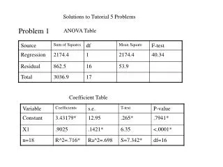
Solutions to Tutorial 5 Problems Problem 1 ANOVA Table Coefficient Table
The Full Medel for (a),(b), and (c ) Results for: P081.txt Regression Analysis: Sales versus Age, HS, Income, Black, Female, Price The regression equation is Sales = 103 + 4.52 Age - 0.062 HS + 0.0189 Income + 0.358 Black - 1.05 Female - 3.25 Price Predictor Coef SE Coef T P Constant 103.3 245.6 0.42 0.676 Age 4.520 3.220 1.40 0.167 HS -0.0616 0.8147 -0.08 0.940 Income 0.01895 0.01022 1.85 0.070 Black 0.3575 0.4872 0.73 0.467 Female -1.053 5.561 -0.19 0.851 Price -3.255 1.031 -3.16 0.003 S = 28.17 R-Sq = 32.1% R-Sq(adj) = 22.8% Analysis of Variance Source DF SS MS F P Regression 6 16499.5 2749.9 3.46 0.007 Residual Error 44 34926.0 793.8 Total 50 51425.4
The RM for (b) Regression Analysis: Sales versus Age, Income, Black, Price The regression equation is Sales = 55.3 + 4.19 Age + 0.0189 Income + 0.334 Black - 3.24 Price Predictor Coef SE Coef T P Constant 55.33 62.40 0.89 0.380 Age 4.192 2.196 1.91 0.062 Income 0.018892 0.006882 2.75 0.009 Black 0.3342 0.3121 1.07 0.290 Price -3.2399 0.9988 -3.24 0.002 S = 27.57 R-Sq = 32.0% R-Sq(adj) = 26.1% Analysis of Variance Source DF SS MS F P Regression 4 16465.7 4116.4 5.42 0.001 Residual Error 46 34959.8 760.0 Total 50 51425.4
(d) Regression Analysis: Sales versus Age, HS, Black, Female, Price The regression equation is Sales = 162 + 7.31 Age + 0.972 HS + 0.845 Black - 3.78 Female - 2.86 Price Predictor Coef SE Coef T P Constant 162.3 250.1 0.65 0.520 Age 7.307 2.924 2.50 0.016 HS 0.9717 0.6103 1.59 0.118 Black 0.8447 0.4213 2.00 0.051 Female -3.781 5.506 -0.69 0.496 Price -2.860 1.036 -2.76 0.008 S = 28.93 R-Sq = 26.8% R-Sq(adj) = 18.6% Analysis of Variance Source DF SS MS F P Regression 5 13769.3 2753.9 3.29 0.013 Residual Error 45 37656.1 836.8 Total 50 51425.4
(e) Regression Analysis: Sales versus Age, Income, Price The regression equation is Sales = 64.2 + 4.16 Age + 0.0193 Income - 3.40 Price Predictor Coef SE Coef T P Constant 64.25 61.93 1.04 0.305 Age 4.156 2.199 1.89 0.065 Income 0.019281 0.006883 2.80 0.007 Price -3.3992 0.9892 -3.44 0.001 S = 27.61 R-Sq = 30.3% R-Sq(adj) = 25.9% Analysis of Variance Source DF SS MS F P Regression 3 15594.4 5198.1 6.82 0.001 Residual Error 47 35831.0 762.4 Total 50 51425.4
(f) Regression Analysis: Sales versus Income The regression equation is Sales = 55.4 + 0.0176 Income Predictor Coef SE Coef T P Constant 55.36 27.74 2.00 0.052 Income 0.017583 0.007283 2.41 0.020 S = 30.63 R-Sq = 10.6% R-Sq(adj) = 8.8% Analysis of Variance Source DF SS MS F P Regression 1 5467.6 5467.6 5.83 0.020 Residual Error 49 45957.9 937.9 Total 50 51425.4